
Fixed Cost Variable Cost
The Costs of Production
A firm uses various inputs to produce goods and services. It has to make payments for such inputs. The expenditure incurred on these inputs is known as the cost of production.
The cost of production is vital in the determination of the level of output that a firm produces. If a firm incurs high production costs, then it is forced to produce fewer quantities of goods.
It is important to understand the concept of opportunity cost as it forms the basis of the concept of cost.{" "} Opportunity cost refers to the cost of next best alternative that is forgone. In other words, it is the benefit that an individual could have received but gave it up, to take another course of action.
For example: A person having $10000 can either purchase a computer or a LED TV and not both. If he decides to purchase LED TV, then the opportunity cost of choosing LED TV is the cost of the foregone satisfaction that the person would have got from Computer.

What is a cost?
In economics, Cost refers to the total expenditure incurred by a firm in producing a particular good or a service. Cost includes both explicit and implicit costs.
a. Implicit cost (or{" "} imputed cost): It is an opportunity cost of using a firm’s internal resources which are not accounted for separately as a distinct expense in the firm’s books. In other words, it is an estimated value of the inputs supplied by the owner of a firm himself.
b. Explicit costs: Explicit costs involve obvious cash outflow or money expenditure on inputs or payments made to providers of factor services. For example: wages or salary paid to employees, payment for raw materials etc.
In order to understand the two costs clearly, consider a simple example:
Suppose A is an entrepreneur who is a skilled computer programmer. However, he starts his own bakery. Now, A incurs explicit costs when he buys flour (a raw material) and hires some workers in order to make cookies, cakes etc. Here he incurs costs that have to be accounted in firm’s accounts, and involve money payments (cash outflow).
Being a computer programmer, he could have easily earned at least $500 per hour by providing his programming services. For every hour, he works in his bakery he has to forgo $500 in income. However, this foregone income is also part of his costs. These opportunity costs which do not involve any cash outlay or money payment are called{" "} implicit costs. This opportunity cost of A will not be recorded by the firm’s accountant as a cost to the business.
Difference between Accounting Cost and Economic Cost
Thus, we can say that an economist will measure a firm’s cost of production by adding both explicit as well as implicit costs. He will consider all the opportunity costs when analyzing a firm, whereas an{" "} accountant will take note of only explicit costs that involve money flowing out of the business.
Types of Costs
1. Money cost: Money cost refers to the total money expenses incurred by a firm in the production of a particular good. Their costs, also known as ‘accounting costs’, arise when there is any transaction between a firm and the other parties that involve outflow of money. Production costs like wages, salaries, rent etc. are some of the examples of money cost.
2. Real cost: Real cost refers to the pain, sacrifice, and disutility involved in providing factor services to produce a commodity. Such costs are psychological and thus cannot be accounted in terms of money. For example, physical and mental efforts by labor in doing the work in a factory.
3. Private cost: Private costs for a producer of a commodity or service are the costs of production incurred by him in producing that commodity or service. These are the costs from the business side and not incurred by the society.
4. External costs: External costs are the costs inflicted upon the society arising as a result of a firm’s production process. Such costs are not reflected in a firm’s income statement. For example: A firm causing air pollution.
5. Social cost: Social costs include both private costs borne by firms directly involved in the transaction and external costs borne by the society.
Different Types of Production Cost
Total Fixed Cost (TFC)
Total fixed costs refer to those costs which do not vary directly with the level of output. Such costs are incurred by the firm irrespective of the level of output. Fixed costs remain same, whether output produced is large, small or even zero. Rent of office premises, interest on the loan, the salary of permanent staff, insurance premium etc. are some of the examples of Fixed costs incurred by a firm.
Consider the following schedule and diagram showing TFC.
| Output (in units) | Total Fixed Cost ($) |
|---|---|
| 0 | 20 |
| 1 | 20 |
| 2 | 20 |
| 3 | 20 |
| 4 | 20 |
| 5 | 20 |
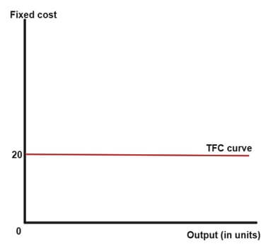
As shown in the figure, Total Fixed cost curve is a horizontal straight-line parallel to X-axis. This is because Fixed cost remains same at all levels of output even if no output is being produced.
The fixed cost is same ($20) for all levels of output. Fixed costs do not vary with the level of output as a firm cannot have half a permanent staff or half a telephone (rent of telephone is a fixed cost) just because it is operating at a low level of output.
Total Variable Cost (TVC)
Total variable costs or variable costs are those costs which vary directly with the level of output. This means that high variable costs have to be incurred at a high level of output and vice versa. Such costs are incurred only when there is the production of a commodity and hence are avoidable. This means variable costs become zero at zero level of output.
Variable factors such as raw materials, wages of casual labor, power etc. are some of the examples of variable costs.
Consider the following schedule and diagram showing TVC:
| Output (in units) | Total Variable cost ($) |
|---|---|
| 0 | 0 |
| 1 | 6 |
| 2 | 10 |
| 3 | 15 |
| 4 | 24 |
| 5 | 35 |
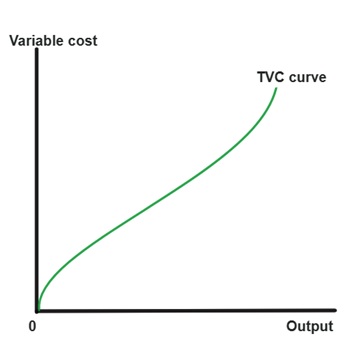
TVC curve is inversely S-shaped. The curve starts from the origin indicating that when output is zero, variable cost is also zero. Initially, the variable cost of firm increases at decreasing rate and at higher levels of output it increases at increasing rate.
Total cost (TC)
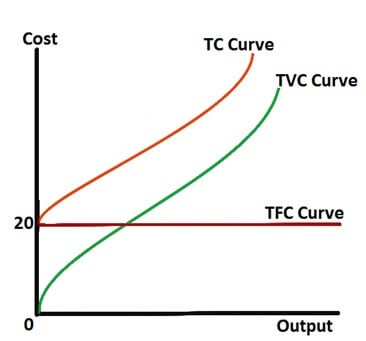
Total cost is the total expenditure incurred by a firm on the factors of production required for the production of a commodity. Total cost is the sum of total fixed cost and total variable cost at different levels of output.
TC=TFC+TVC
As TFC remains same at all levels of output, the change in TC is only due to TVC.
Consider the following schedule and diagram showing TVC:
| Output (in units) | Total Fixed Cost ($) | Total Variable cost ($) |
Total cost (TC)
[TC=TFC+TVC] |
|---|---|---|---|
| 0 | 20 | 0 | 20 |
| 1 | 20 | 6 | 26 |
| 2 | 20 | 10 | 30 |
| 3 | 20 | 15 | 35 |
| 4 | 20 | 24 | 44 |
| 5 | 20 | 35 | 55 |
Like TVC, TC is also inversely S-shaped curve. This is because the change in TC is only due to changes in TVC i.e. the shape of TC curve is derived from the shape of TVC curve.
At zero level of output, TC is equal to TFC because no variable cost is incurred at zero level of output. TC and TVC curves are parallel to each other and the vertical distance between the two curves is TFC which remains same at all levels of output.
Average Fixed cost (AFC)
Average fixed cost refers to the per unit fixed cost of production. It can be calculated by dividing Total fixed cost (TFC) by total output. AFC can be mathematically expressed as:
AFC = TFC/Q
Consider the following schedule and diagram showing TVC:
| Output (in units) | Total Fixed Cost ($) | Average Fixed Cost ($) |
|---|---|---|
| 0 | 20 | 20/0=∞ |
| 1 | 20 | 20/1=20 |
| 2 | 20 | 20/2=10 |
| 3 | 20 | 20/3=6.67 |
| 4 | 20 | 20/4=5 |
| 5 | 20 | 20/5=4 |
AFC curve is downward sloping as AFC falls with an increase in the level of output. This is because TFC remains fixed at all levels of output. The shape of the AFC curve is of a rectangular hyperbola. The area under the curve remains same at all points.
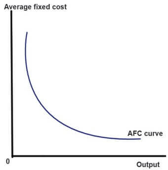
AFC never touches the axis of XY plane. AFC can never touch X-axis as TFC can never be 0.AFC cannot touch Y-axis as at zero level of output, TFC is a positive value. Any positive value, when divided by 0, will give an infinite value.
Average Variable Cost (AVC)
Average variable cost refers to per unit variable cost of production. AVC is TVC divided by total output. AVC can be mathematically expressed as:
AVC = TVC/Q
| Output (in units) | Total Variable cost ($) | Average Variable Cost ($) |
|---|---|---|
| Output (in units) | Total Variable cost ($) | Average Variable Cost ($) |
| 0 | 0 | - |
| 1 | 6 | 6/1=6 |
| 2 | 10 | 10/2=5 |
| 3 | 15 | 15/3=5 |
| 4 | 24 | 24/4=6 |
| 5 | 35 | 35/5=7 |
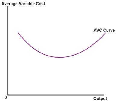
As is shown in the figure, AVC initially falls as the output increases. Once the output rises till optimum level, AVC starts rising again. Thus, AVC is a U-shaped curve.
Average Total Cost (ATC)
Average Total Cost refers to the per unit total cost of production. ATC is the Total cost (TC) divided by the total quantity of output. ATC can be mathematically expressed as:
ATC=TC/Q
As Total cost is the sum of total fixed cost and total variable cost, the average total cost can also be expressed as the sum of average fixed cost and average variable cost.
ATC=AFC+AVC
| Output (in units) | Average Fixed Cost ($) | Average Variable Cost ($) | Average Total Cost ($) |
|---|---|---|---|
| 0 | 20/0=∞ | - | - |
| 1 | 20/1=20 | 6/1=6 | 20+6=26 |
| 2 | 20/2=10 | 10/2=5 | 10+5=15 |
| 3 | 20/3=6.67 | 15/3=5 | 6.67+5=11.67 |
| 4 | 20/4=5 | 24/4=6 | 5+6=11 |
| 5 | 20/5=4 | 35/5=7 | 4+7=11 |
| 6 | 20/6=3.33 | 47/6=7.83 | 3.33+7.83=11.16 |
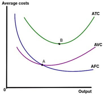
As is clear from the diagram, AC curve always lies above the AVC curve. This is because, at all level of output, ATC includes both AVC and AFC.
AVC curve reaches its minimum at point A while ATC reaches its minimum at point B. AVC has its minimum at a lower level of output than of ATC because when AVC reaches its minimum point, ATC is still falling because of falling AFC.
Marginal Cost (MC)
Marginal cost refers to addition to the total cost when one more unit of output is produced. It can be expressed mathematically as:
Marginal cost=(change in total cost)/(change in quantity)
MC=∆TC/∆Q
Where ∆ represents the change in a variable
| Output (in units) | Total Variable cost ($) | Total Fixed Cost ($) | Total cost (TC) | Marginal Cost (MC) |
|---|---|---|---|---|
| 0 | 0 | 20 | 20 | - |
| 1 | 6 | 20 | 26 | (26-20)/(1-0)=6 |
| 2 | 10 | 20 | 30 | (30-26)/(2-1)=4 |
| 3 | 15 | 20 | 35 | (35-30)/(3-2)=5 |
| 4 | 24 | 20 | 44 | (44-35)/(4-3)=9 |
| 5 | 35 | 20 | 55 | (55-44)/(5-4)=11 |
The graph shows the relation between Marginal cost of a firm and the level of output produced.
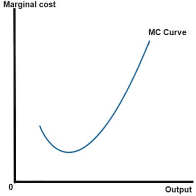
Marginal cost curve, as shown, is a U-shaped curve. The MC curve initially falls till it reaches its minimum point and finally rises.
Initially, at lower levels of output, a firm experience increasing marginal productivity (increasing marginal returns), and as a result, the Marginal cost falls. Gradually, the firm starts to experience diminishing marginal product (due to the law of diminishing marginal returns) and Marginal cost eventually rises with an increase in the level of output.
Relationship between Marginal cost (MC) and Average total cost curves (ATC)
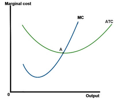
Marginal cost and Average total cost display an important relationship. The relationship between the two costs can be summarized as follows:
- When MC is less than ATC (MC < ATC), then ATC falls with an increase in the level of output.
- MC curve and ATC curve intersect each other ( MC = ATC) at point A, which is the point at which Average total cost is minimum. Thus, MC intersects the ATC curve at the minimum point of Average total cost curve (ATC).
- When MC is higher than ATC (MC > ATC), then AC rises with an increase in the level of output.
Long Run and Short Run Average Total Cost Curves
All the cost functions that we discussed above were{" "} short run cost functions. In short run, output can be changed only by changing variable factors. On the other hand, in long run period, the output can be changed by changing all factors of production.
In brief, in long run, all the factors are classified as a variable while factors are classified as variable and fixed in short run.
For example, consider a car manufacturing company who wants to increase its car production in short period, say in a period of few months. In short run, the manufacturer cannot increase the number of car factories. The only way the company can increase its car production is by hiring more workers at the existing factories. Thus, in short run, the cost of the factories is fixed cost while the cost of hiring workers in variable cost (which is used to increase car production in short run). However, in long run, the car manufacturer can sell old factories, build new factories and thus expand its factory size in order to increase the level of production. thus, in long run, the cost of factories become variable and can be used to increase output. The decision that was fixed in the short run became variable in the long run. This is the reason why a firm’s long run cost curves differ from short run cost curves.
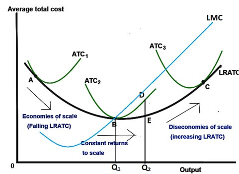
As shown in the figure, there are 3 short run average total cost curves - ATC1, ATC2 and ATC3.The long run average total cost (LRATC) curve is flatter than the short run ATC curves. All the short run ATC curves lie on or above the LRATC curve.
Suppose a manufacturer of the car (who is currently operating at short run ATC2 curve) wants to increase the production from Q1 to Q2. As discussed before, in the short run, he has no option, but to hire more workers at the existing factory size. As the level of cars produced increases to Q2, the average total cost also increases to D{" "} due to the law of diminishing returns. However, in the long run, the manufacturer has greater flexibility. He can expand both the workforce and the factory size in order to increase production level. In this case, the average cost comes down to point E.
The long run Average total cost curve shows us how costs to the firm vary with its scale of production.
Economies of scale
When long run Average Total Cost curve falls as output increases, then the firm is said to be operating at economies of scale. Economies of scale arise when a higher level of production allows specialization of workers which allow each worker to become an expert in a particular work. For instance, in the long run, as the car manufacturing company produces more cars with more number of workers, it can reduce LRATC by assigning specific tasks to each worker.
Constant returns to scale
When Long Run Average total Cost Curve does not vary with changes in output level, then the firm is said to be operating at constant returns to scale. The car manufacturer whose LRATC and Short run ATC curves are depicted in the figure, is facing constant returns to scale.
Diseconomies of scale
When Long Run Average Total Cost curve rises as output increases, then the firm is said to be operating at diseconomies of scale. Diseconomies of scale arise when there are severe coordination problems in a large-scale organization. As a company and its management grow in size, it becomes difficult to keep the costs down.
Economies of scale, as shown in the figure, arises at the lower level of output, constant returns to scale arises at the intermediate level of output and diseconomies of scale occurs at the higher level of output.
As in the case of short run, long run marginal cost also intersects the Long Run Average total cost at the minimum of LRATC. In the above figure, LMC curve will intersect LRATC curve at point B. Also note that at point B,{" "} ATC2 = LRATC .
Online Microeconomics Homework Help
Looking for help with your Microeconomics Problem Set on topics like Cost Curves, Production Theory, Market Structures, Perfect Competition, Monopoly, Opportunity Costs and Scarcity and much more? Urgenthomework.com is the best online website for Microeconomics homework help. Whether it is basic homework assignment work on principles of Microeconomics or advanced Microeconomics theory, our{" "} online economics homework tutors {" "} have mastery over all basic, intermediate and advanced economics concepts and are best options for online economics tutoring, economics research writing, economics academic help and economics homework help.{" "} So, hurry up and order your economics homework help assignments writers now!
Important topics in Economics
- Behavioral Economics
- Cost of Production
- Derivatives Market
- Economic Growth
- Economic Systems
- Efficiency
- Game theory
- Inflation
- International Economics
- Macroeconomics
- Market failure
- Marxism
- Microeconomics
- Monopoly
- Normative Economics
- Price Elasticity of Demand
- Revenue
- Supply and demand
- Welfare Economics
- Scarcity
- Specialization
- Classical theory
- Depression and unemployment
- Development Economics
- Economic thought
- Managerial Economics
- Public Economics
