
Database and data science techniques
INTRODUCTION TO THE DATABASE:
Database is a collection of information that is organized so that it can be easily accessed, managed and update whenever we need it. Data is information that is collected in the form of tables organized into rows and columns; it can take numeric or alphabetic form based on collection process and objective of data. We know data can be static and dynamic in nature depending on the type of data. Hence, new updates in data needs more organized way so they can be easily traceable and informative; we use computer techniques and programming to evaluate the organized data which is not possible with unorganized data set. Database can be in different forms such as graphical database, object-oriented database, cloud database, or distributive database etc. To get a proper database we require data cleaning so we can increase the quality of data predictability.
For our purpose we will use data that we have from 178 countries and number of mammals present who are under threat of extinction, there are few factors which are responsible for their extinction. Some of them are including a number of mammals with extinction:
                    Mammals: Mammal species threatened with extinction CO2EM:
                    CO2 emissions (metric tons per capita) Forest: Forest Area
                    (sq. km) Energy: Energy intensity level of primary energy
                    (MJ/$2011 PPP GDP) Gdppc: GDP per capita (constant 2010 US$)
                    Popden: Percentage of population in areas with elevation
                    below 5 meters (%) Access: Percentage of population with
                    access to non-solid fuels (%)
USE OF DATA SCIENCE TECHNIQUES:
We have already defined what is the database? Why do we need this? Now, we can talk about some data science techniques that will be used to exploit database and come out with some reasonable conclusions.
Data techniques: Data techniques are the statistical techniques that we do use some statistical packages like EXCEL,{" "} Matlab , R and STATA.

CORRELATION:
Correlation analysis is a method of statistical technique used to study the strength of the relationship between two variables. It is used when researchers want to know is there any possible connection between these variables or not? It is nothing to do with the causal effect, it only tells about the connection between these variables. If a correlation exists then it says that there is a systematic change in variables. It is measured by numerical values ranging from -1 to 1, former suggest about the perfect negative relationship and later suggesting a perfect positive relationship. If correlation numerical values are 0 then we can say there is the absence of systematic change between variables. We can calculate the correlation coefficient between two variables for our data.
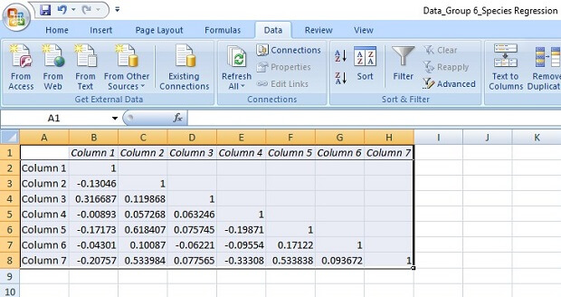
From the result, we can say that there is a strongest positive relationship between co2em and gdppc and strongest negative relationship between mammals and access to another variable. There is a property of correlation that it always carried value 1 whenever we calculate it for the same variable.
LINEAR REGRESSION IN ONE/MULTIPLE VARIABLES:
There is always some relationship between variables it may be positive, negative and zero. They have a causal effect or not it may be debatable but they have some correlation ranging from -1 to 1. We use the statistical technique to find out the relationship between dependent (target) variable and independent variables which are known as the linear regression. It has some general form as
Y= α1i+a2i*X2i+a3i*X3i+⋯+ani*Xni+ui
Where a1i is an intercept, aji are coefficient of variables except j=1, Y is a dependent variable, Xji are independent variables and ui is one of the most important term in linear regression modeling. We have certain set of assumption to apply the particular type of modeling and estimate the parameters. For linear regression model which is satisfying Guasian assumptions, we rely on the OLS (ordinary least square) method to for best estimation the parameters.
DATA ANALYSIS FOR OUR DATA SET:
Primarily data is highly right skewed and with high kurtosis for each variable and most concerning with popden variable which has its 95% value below the 1752.503 but after that its value is shooting up and ended with 7636.721. Access is the only variable which shows negative skewness. The conclusion is that most of the data is away from the mean value of the respective variable.
This can be easily observable through the kdensity, normal comparison. Data also do not have any missing values for any of the variable’s entry. Hence ones we do not have any problem with data we can easily move into the regression analysis which is the main objective of our analysis.
REGRESSION ANALYSIS
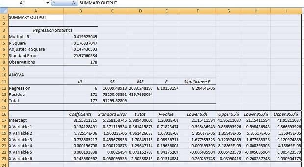
Now we regress the data of mammals with the respective independent variables we get the following analysis for data. As we look to the p-value of the F-test to see which is zero to four decimal places, the model is statistically significant. The R-squared is 0.1763, meaning that approximately 17.63% of the variability of{" "} mammals is accounted for by the variables in the model. In this case, the adjusted R-squared indicates that about 14.74% of the variability of{" "} mammals is accounted for by the model, even after taking into account the number of predictor variables in the model. The coefficients for each of the variables indicates the amount of change one could expect in{" "} mammals given a one-unit change in the value of that variable, given that all other variables in the model are held constant. For example, consider the variable{" "} CO2em . We would expect an increase of 0.1341 in the mammals for every one unit increase in CO2em, assuming that all other variables in the model are held constant. Similarly, for other, Variables{" "} energy, gdppc, and access have a negative relationship with mammals.{" "} P-values of the beta coefficient are insignificant for the variable co2em, energy, gdppc, and{" "} popden because it has value more than 0.05. that is major concerning.
We can also calculate the strength of the coefficient of the variable, which is independent within the model. When we do that then we get that unit increase in the standard deviation of CO2em leads to a 0.0358 sd increase., unit increase in the sd of{" "} forest leads to a 0.3486 sd increase,
unit increase in the sd of energy leads to a 0.1347 sd decrease, unit increase in the sd of{" "} gdppc leads to a 0.1234 sd decrease, unit increase in the sd of popden leads to a 0.005 sd increase, unit increase in the sd of{" "} access leads to a 0.2331 sd increase. These results are units unaffected.
P-value of F-test is zero up to four decimal places which represent that model is statistically significant.
After computing the residual when we checked it then we got that residual is also abnormal and it is far away from the normal. Normality of residuals is the most important assumption in an OLS regression model.
On analyzing the correlation of{" "} mammals with the predictor variables then we get that no any variable has a significant correlation with mammals hence there is no indication that any variable may play the significant role of to analysis the effect on mammals.
To analysis the regression model we need to fulfill all the assumption of OLS model. The first and most assumption is the normality of residual term and predicator variables along with the dependent variable. We have already seen that most of our variable are skewed and have high kurtosis hence there nonnormality is an exit. Now our aim is to transform all the predictor variables and make them satisfy the assumption of normality.
Values for mammals, CO2em, forest, gdppc, energy, popden, and access are skewed either negative or positive. Similarly, Kurtosis is also abnormal. Hence we can transform these variables to achieve the best normality assumption such as
                    TRANSFORMING VARIABLES VARIABLE ~ TRANSFORMED VARIABLE
                    Mammals ~ (mammals)^1/4 CO2em ~log10 (CO2em) Forest
                    ~(forest)^1/8 Energy ~1/sqrt*(energy) Gdppc ~log10 (gdppc)
                    Popden ~ log10 (popden) access ~sprt(access)
These transformations are the best possible normal for the model. When we regress these variables then we will get a more fruitful result:
Analysis of transformed model
It gives us some improved model which is statistically significant because it has P-value of F-test is zero to the four decimal places. R2 has been increased from .1763 to .5303 that means now 53.03% variability of mammals is accounted for by the variables in the model.
Adjusted R2 has also increased significantly from .1474 to .5138. It also shows that MSE has also reduced from20.971 to .35204. Now we can interpret changed variable coefficient as that unit increases in the transformed predictor variables co2em, forest, energy, gdppc, popden, access leads to the .3458, .2988, .9618, -.4866, .1155 and -.03739 changes in transformed dependent variable. Now intercept constant also has been reduced from 31.55 to 2.12. This result is also showing that all the p-values are significant except sqrt (access) variable which still has p-value.
The transformed model does not have heteroscedasticity because #estate hettest H0= homoscadesticity against Ha= heteroscedasticity gives the p-values which are insignificant.
Transformed model is also multicollinearity free it can be shown by using a command of #vit if stata . Every predictor variable has VIF which is less than 10 which is not a concern.
But the model has some specification biasedness because it fails on #ovtest where p-values which is less than 0.05. But this specification bias of omitted variable was present in the original model too. Hence we can conclude that for best prediction we need some of more variables which are responsible for no. of mammals with extinction.
But overall transformed model is the far better than the untransformed model because it has high R2, adjusted- R2 and more significant p-values.
MODEL AND ITS INTERPRETATION
This model shows that no. of mammals species with endangered are affected by the emission level of carbon dioxide which seems reasonable because CO2em is harmful not for only mammals but it is for all. It shows that as the gdppc increase then the no. of mammals with endangered decrease perhaps it would be due the fact the when gdppc increased then country have more enough recourse to provide a safe environment for these mammals. It also supports the study that endangerment of species and gdppc have u shaped the relationship.
HYPOTHESIS TESTING:
Researchers are more interested in hypothesis methodology as they want to check weather their resulted parameters are fitting with the hypothesis test or not. They use this technique to reject or do not reject the null hypothesis that is set by the observer. Researchers find out a confidence interval using a type of data and statistical tables. Parameter values that lie within the confidence interval known as acceptance region are given confidence to the researcher that they test are likely to satisfy the standard. If calculated parameter values lie outside of the confidence interval then researchers usually reject the null hypothesis. Null hypothesis and alternative hypothesis usually represented by.
DECISION TREES:
A decision tree is a graph starting with a nod; it consists of branches those represent the decisions taken place by players of the game. It may be static or strategic. It helps us to know which decision can be taken by whom and who is likely to gain and loose from the corresponding decision. We assign some numerical values for outcomes so that decision can be automated. Generally, we use{" "} data tree software for data mining to simplifying complex strategic challenges and evaluate the effectiveness of models. Variables in the Decision tree are usually representing by circle nodes.
Decision tree applications play important role in the model that is in game theory where a decision taken by one firm affects the decision by other firms. And each decision has its own impact for all the members in the game.
Although, this data set is not very suitable to discuss decision tree since it is not strategic and player game. In our data set, we can choose countries those have less and more co2em values than its mean value. Then we can follow the next step as what is the effect on a number of mammals in both the groups. Since co2em is the variable which has repercussion effect for all the countries including itself. So we can formulate the model as following,
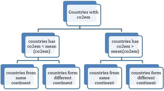
To know the effect of the decision taken by one group of the country on the other is we can estimate the parameters again and see the results. We have to just separate out these groups using data mining techniques.
Limitations: Along with this subject, we might have missed out some important variables that may lead to the omitted variable biasness in our estimation for parameters. Some of the results seem very obvious to us. As we did use every precision technique to rule out any inconsistency in our project, even we will talk in probability term. We cannot be sure by 100% in our results.
Conclusion: The database is the best way to organize the data by doing{" "} Data Mining . We can always use data science techniques to get some positive results which may help us to find out solutions for them. Specification of the model is an important technique that we can use to make a complex problem simple linear regression form, which is easy to handle conceptually.
Appendix:
Sources:
Wikipedia
“Basic econometric” for the graduate student by Gujarati.{" "}
Excel Commands:
Correlation:
>>Data>>Data
analysis>>correlation>>select tables{" "}
Regression:
>>Data>>Data
analysis>>regression>>select tables
Topics in database
- Authorization: SQL Recursion
- Big Data
- Database and data science techniques
- Database Languages Assignment Help{" "}
- Database Design Help
- Database System Architectures Design
- Entity Relationship Model Understanding
- Higher-Level Design: UML Diagram Help
- Implementation Of Atomicity And Durability{" "}
- Object-Based Databases Homework Help
- Oracle 10g/11g
- Parallel And Distributed Databases
- Query Optimization Technique{" "}
- {" "} Relational Databases Homework Help
- Serializability And Recoverability
- SQL Join
- SQL Queries And Updates
- XML And Relational Algebra Homework Help
- XML Queries And Transformations
- Data Mining
- Oracle Data warehouse
- Relational Model Online Help
- SQL And Advanced SQL Learning Help
