
Amsi associate professor david hunt
Limits and continuity
Limits and continuity – A guide for teachers (Years 11–12)
Full bibliographic details are available from Education Services Australia.
Published by Education Services Australia
PO Box 177
Carlton South Vic 3053
Australia
Australian Mathematical Sciences Institute
Building 161
The University of Melbourne
VIC 3010
Email: enquiries@amsi.org.au
Website: www.amsi.org.au
Links forward . . . . . . . . . . . . . . . . . . . . . . . . . . . . . . . . . . . . . . . . . . 18 Formal definition of a limit . . . . . . . . . . . . . . . . . . . . . . . . . . . . . . . . 18 The pinching theorem . . . . . . . . . . . . . . . . . . . . . . . . . . . . . . . . . . . 19 Finding limits using areas . . . . . . . . . . . . . . . . . . . . . . . . . . . . . . . . . 20
History and applications . . . . . . . . . . . . . . . . . . . . . . . . . . . . . . . . . . . 21 Paradoxes of the infinite . . . . . . . . . . . . . . . . . . . . . . . . . . . . . . . . . . 21 Pi as a limit . . . . . . . . . . . . . . . . . . . . . . . . . . . . . . . . . . . . . . . . . 22 Infinitesimals . . . . . . . . . . . . . . . . . . . . . . . . . . . . . . . . . . . . . . . . 22 Cauchy and Weierstrass . . . . . . . . . . . . . . . . . . . . . . . . . . . . . . . . . . 22
Assumed knowledge
The content of the modules:
Motivation
Functions are the heart of modelling real-world phenomena. They show explicitly the relationship between two (or more) quantities. Once we have such a relationship, various questions naturally arise.
Both of these examples involve the concept of limits, which we will investigate in this module. The formal definition of a limit is generally not covered in secondary school
Limit of a sequence
Consider the sequence whose terms begin
| � 1 n: n = 1,2,3,... | � | |||
|---|---|---|---|---|
|
|
|||
for any positive real number a. We can use this, and some algebra, to find more compli-cated limits.
A guide for teachers – Years 11 and 12 • {7}
|
|
|---|
This generates the sequence
{8} • Limits and continuity
A typical geometric sequence has the form
a,ar,ar2,ar3,...,arn−1
| Sn =a(1−r n) 1−r |
|
|
|---|
A guide for teachers – Years 11 and 12 • {9}
| 0 |
|
|---|
We write
f(x)
2
| 0 | x |
|---|
{10} • Limits and continuity
| lim | 2 | ||
|---|---|---|---|
| x→∞ | 1+ x2 = lim x→∞ |
Note that as x goes to negative infinity we obtain the same limit. That is,
x(t) = Ae−αtsinβt,
where A, α and β are positive constants. The factor Ae−αtgives the amplitude of the motion. As t increases, this factor Ae−αtdiminishes, as we would expect. Since the factor sinβt remains bounded, we can write
For example, as x gets close to the real number 2, the value of the function f (x) = x2gets close to 4. Hence we write
x→2x2 = 4.
y
| –5 | –4 | –3 | –2 | –1 | 0 | 1 | 2 | 3 | 4 | 5 | |
|---|---|---|---|---|---|---|---|---|---|---|---|
We can see from the ‘jump’ in the graph that the function does not have a limit at 2:
• as the x-values get closer to 2 from the left, the y-values approach 5
• but as the x-values get closer to 2 from the right, the y-values do not approach the same number 5 (instead they approach 2).
{12} • Limits and continuity
Now, when x is near the value 3, the value of f (x) is near 3 + 3 = 6. Hence, near the x-value 3, the function takes values near 6. We can write this as
|
|||
|---|---|---|---|
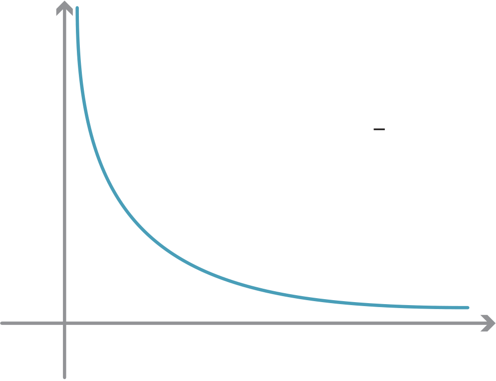
is not defined at the point x = 1. As x takes values close to, but greater than 1, the values of f (x) are very large and positive, while if x takes values close to, but less than 1, the
values of f (x) are very large and negative. We can write this as
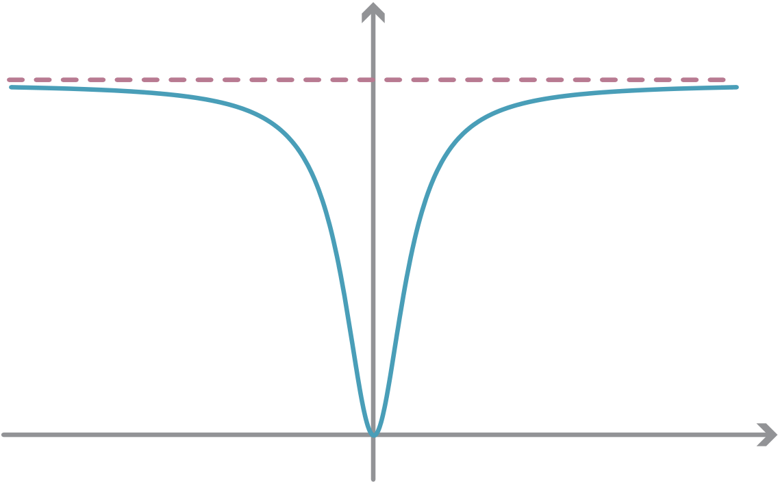
y = 0 is a horizontal asymptote.
y
| 0 | 1 | x |
|---|
Discuss the limit of the function
|
|---|
|
� |
|
|---|
Exercise 6
| Find | ||||||
|---|---|---|---|---|---|---|
| a | lim x→1 | � | b | lim x→4 | ||
Algebra of limits
Suppose that f (x) and g(x) are functions and that a and k are real numbers. If both
b x→ak f (x) = k lim x→af (x)
c x→af (x)g(x) =�x→af (x)��x→ag(x)�
Continuity
When first showing students the graph of y = x2, we generally calculate the squares of a number of x-values and plot the ordered pairs (x, y) to get the basic shape of the curve. We then ‘join the dots’ to produce a connected curve.
Here are more examples of functions that are continuous everywhere they are defined:
if x = 3. |
|||
|---|---|---|---|
| (x −3)(x +3) x −3 | |||
Since 6 is also the value of the function at x = 3, we see that this function is continuous. Indeed, this function is identical with the function f (x) = x +3, for all x.
Now consider the function
7 (3,7)
3
| –3 | 0 | 3 | x |
|---|
• f (a) is defined, and
• x→af (x) = f (a).
5 4 |
d g |
to look at the limit from the right-hand side x −2 and so
|
||||
|---|---|---|---|---|---|---|
–1 –2 |
Exercise 7
Examine whether or not the function
Links forward
Formal definition of a limit
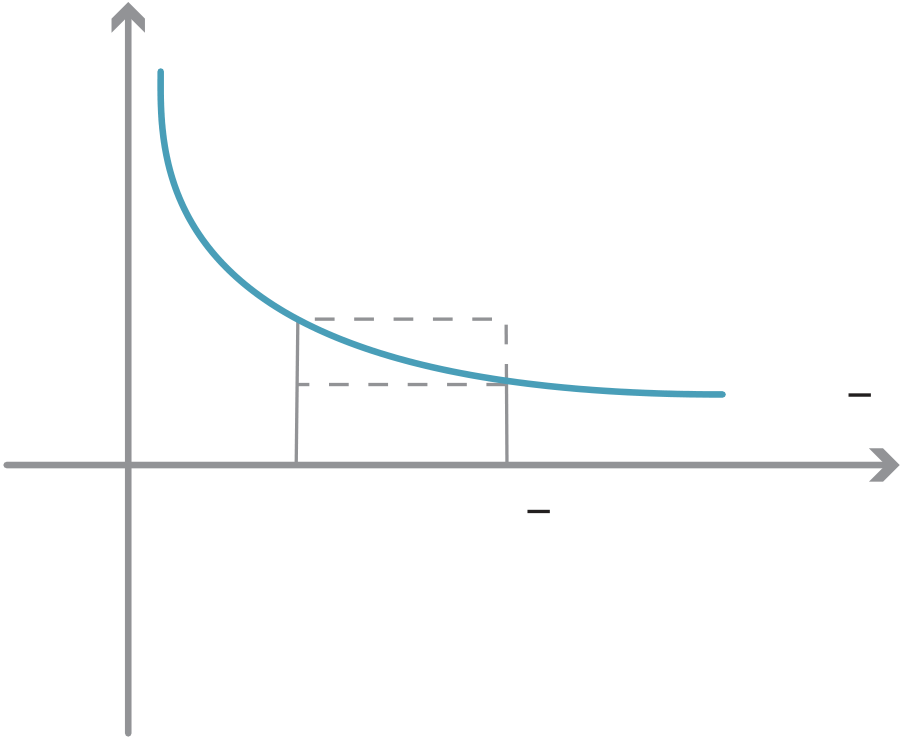
The formal definition of lim x→∞f (x) = L is that, given any ε > 0, there is a number M such that, if we take x to be larger than M, then the distance |f (x)−L| is less than ε.
y
| 0 | x |
|---|
The value of f (x) stays within ε of L from the point x = M onwards.
y
1 + ε
While the formal definition can be difficult to apply in some instances, it does give a very precise framework in which mathematicians can properly analyse limits and be certain about what they are doing.
The pinching theorem
{20} • Limits and continuity
Here is a simple example of this.
| nn = n n× n −1 | ×n −2 | ||
|
|||
y
| 0 | 1 | 1+1 n | f(x) = | 1 x |
|
|---|
Hence
|
�1+1 | � |
|---|
Paradoxes of the infinite
The ancient Greek philosophers appear to have been the first to contemplate the infinite in a formal way. The concept worried them somewhat, and Zeno came up with a number of paradoxes which they were not really able to explain properly. Here are two of them:
In both of these supposed paradoxes, the problem lies in the idea of adding up infinitely many quantities whose size becomes infinitely small.
{22} • Limits and continuity
2����1 2+ 1�2+ 1�1 |
|---|
He also introduced the symbol ∞ into mathematics.
Infinitesimals
Cauchy and Weierstrass
Prior to the careful analysis of limits and their precise definition, mathematicians such as Euler were experimenting with more and more complicated limiting processes; some-times finding correct answers — often for wrong reasons — and sometimes finding in-correct ones. A lack of rigour often led to paradoxes of the type we looked in the section Paradoxes of the infinite.
Analysis may be thought of as the theoretical side of limits and calculus. It is a very important branch of modern mathematics, and teaches us how to deal with calculus in ways that are rigorous and logically valid.
In 1821, Cauchy wrote Cours d’Analyse, which had a great impact on continental math-ematics. In it he introduced proofs using the ε notation we saw in the section Links forward (Formal definition of a limit).
f(a)
f(a) –ε
| 0 | a – δ | a | x |
|---|
This basically says that a function f (x) is continuous at a point a if x-values that are close to a (i.e., within δ of a) get mapped by f to y-values that are close to f (a) (i.e., within ε of f (a)).
In fact, this definition of the continuity of f (x) at a says exactly that lim using the formal definition of a limit. So it agrees with our definition of continuity in the x→af (x) = f (a),
| 1 | 2 | 3 | 4 | 5 | 6 |
|---|
quickly approaches 0 as n gets larger. It is this aspect that is used to prove continuity. It can be formally proven that the infinite series converges for every value of x, and that the function so generated is continuous everywhere. If, however, we were to try to differen-tiate this function term-by-term, then the derivative of the general term is −2nsin(4nx) whose amplitude is 2n, which becomes very large as n increases. So the series of deriva-tives does not converge. Hence the function is not differentiable anywhere.
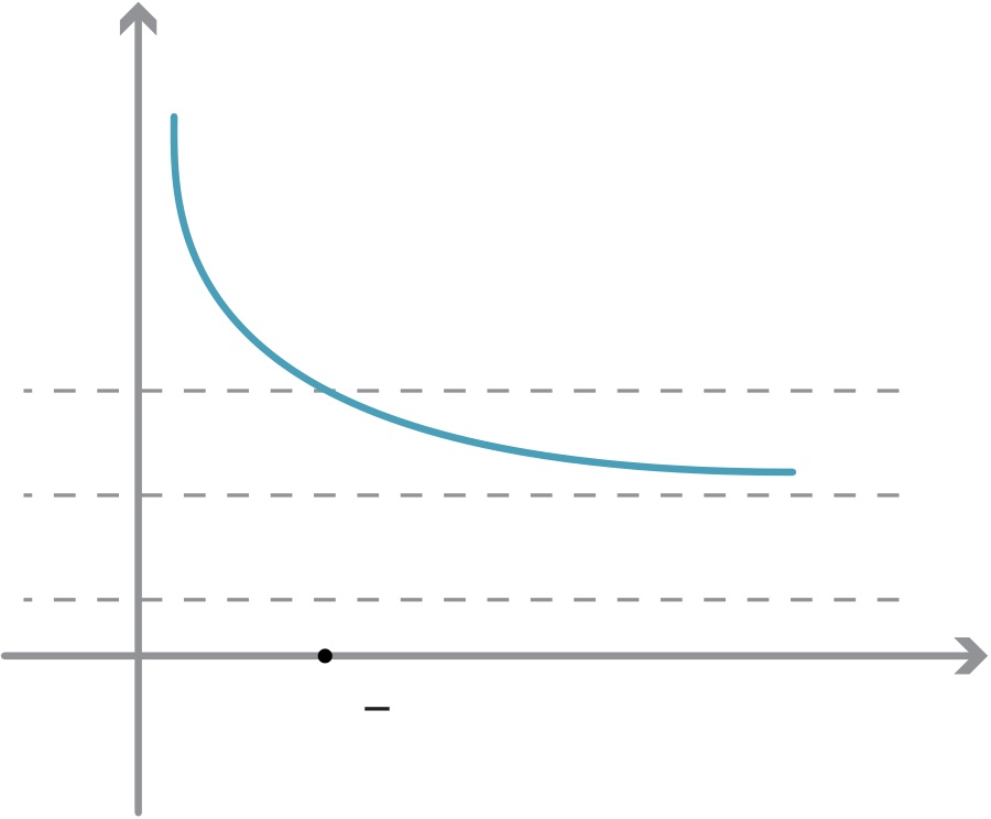
| 5n3+(−1)n 4n3+2 | = lim n→∞ | 5+(−1)n 4+2 n3 |
|
|---|
Exercise 2
Exercise 3
|
|||
|---|---|---|---|
|
|||
Exercise 4
| a |
|
||
|---|---|---|---|
| b |
|
||
| c | |||
| d | +, and f (x) → +∞ as x
→ |
||
| e | |||
Exercise 6
Exercise 7
ε. Hence, we take M =� |
|---|
The following introductory calculus textbook begins with a very thorough discussion of functions, limits and continuity.
• Michael Spivak, Calculus, 4th edition, Publish or Perish, 2008.