
Analyze the results usingthe kpi dashboard revenue
Level 2 Advanced
Prof. Dr. Dmitry Ivanov
© Prof. Dr. Dmitry Ivanov, 2021. All rights reserved.
0
anyLogistix has become more and more popular with the provision of the free PLE version, and because it is an easy-to-use software, includes simulation and optimization, and covers all standard teaching topics (center-of-gravity, efficient vs responsive SC design, SC design through network optimization, inventory control simulation with safety stock computations, sourcing (single vs. multiple) and shipment (LTL vs FTL) policy simulation, and milk-run op-timization). This guide has been developed to support a course in Supply Chain Optimization and Simulation using anyLogistix software using two sample project reports. The following themes will be considered:
•Facility Location Planning (COG, Trade-off Efficiency vs Responsiveness) •Supply Chain Design (Network optimization, CPLM)
•Inventory Control Policy (simulation, safety stocks, ordering policies) •Sourcing Policy (simulation, single vs multiple sourcing)
•Shipment Policy (LTL/FTL, aggregation rules)
Upon completing the course, students should be able to do the following:
•Develop critical thinking skills, be able to identify, generalize, prioritize, isolate, and reduce complexity in complex and ambiguous operational situations,
•Understand how strategic considerations influence operational decisions,
•Apply analysis and improvement tools learned in previous courses to actual business situations,
•Strengthen qualitative and quantitative reasoning skills for operational decision-making.•Building a new SC from scratch - a case study of the Polarbear Bicycle company, which must create and optimize its SC in order to maintain profitability and keep its competitive edge in an increasingly global market where sales prices are driven down while costs re- main stable and
•Improving the existing SC - a case study of the beer producer BERLIN BREWERY, which seeks to analyze the performance of their existing SC and optimize its distribution network, while considering the risks and ripple effect.Using the models available in anyLogistix, we will conduct analyses to (1) determine an optimal location using Greenfield Analysis (GFA) for a new warehouse, given the location of their cur-rent customers and those customers relative demands, (2) compare alternative network designs using Network Optimization (NO), (3) perform a Simulation of different scenarios, (4) validate
2. Case study 1
2.1 Description of Case Study
2.2 Greenfield Analysis (GFA) for Facility Location Planning: Selecting the Best
Warehouse Location for Polarbear Bicycle
|
|---|
|
|---|
|
|---|
|
|---|
After selling the bicycles from the newly established DC according to the GFA results, Polar-bear decided to produce their own bicycles. Their production facility has now been established in Nuremberg and 250 bikes are produced each day. Recently, they have received an offer from a Polish production factory to rent a DC in the Czech Republic at a reasonable price. The same company also wants to offer them rental of a factory in Warsaw, Poland, even though they already have one factory in Germany. Polarbear must now decide which SC design is more profitable:
•Option 1: DC in Germany and Factory in Germany
•Option 2: DC in Germany and Factory in Poland
•Option 3: DC in Czech Republic and Factory in Poland •Option 4: DC in Czech Republic and Factory in GermanyTherefore, the factory in Warsaw, Poland, the DC in the Czech Republic, and the DC in Steim-elhagen were added as inputs to the model along with the Nuremburg factory. To enable the model’s calculation, the reality of the case must be simplified: all demand is assumed to be deterministic without any uncertain fluctuations. To define the two-stage NO problem (transport between factories and DCs and between DCs and customers) from a mathematical perspective, several parameters must be input as data. These are shown in Table 2.
7
| Costs | Value in USD |
|---|---|
| 15,000 | |
| 5,000 | |
| 15,000 | |
| 3.00 | |
|
5,000 |
|
2.00 |
| 2.00 | |
| 1.00 | |
| 250 | |
| 150 | |
|
30 |
|
|
| 499 |
Table 2. Cost inputs to optimization model
The costs of the rent for the factory in Poland and the DC in Czech Republic are included in “other costs”. For transport, it is always assumed that each truckload fits 80 bicycles, and trucks travel at a speed of 80 km/h.
|
|---|
| Step 1. Go to NO Experiment and run it with the Demand variation type “95-100%”. |
|---|
8
b)Is demand for all customers satisfied?
|
|---|
NOTE! In order to run the NO experiment, units in experiment settings should be aligned
with product data (e.g., m3 and pcs should be used consistently, and unit conversions
each bicycle type within the range of 10,000 units (minimum capacity utilization) and 25,000
units (maximum capacity utilization). Polarbear must now conduction another NO to include
|
|---|
a)What is the most profitable SC design considering the capacity constraint of the factory in Poland?
b)What is the total profit of the most profitable SC?
| Customer | Bicycle Type |
|
|
|---|---|---|---|
| Cologne | x-cross | 2 | - |
| Cologne | urban | 50 | 8 |
| Cologne | all terrain | 15 | 2 |
| Cologne | tour | 10 | 3 |
| Bremen | x-cross | 7 | - |
| Bremen | urban | 30 | 6 |
| Bremen | all terrain | 20 | 5 |
| Bremen | tour | 20 | 3 |
| Frankfurt am Main | x-cross | 6 | - |
| Frankfurt am Main | urban | 5 | - |
| Frankfurt am Main | all terrain | 4 | - |
| Frankfurt am Main | tour | 5 | - |
| Stuttgart | x-cross | 15 | - |
| Stuttgart | urban | 15 | - |
| Stuttgart | all terrain | 1 | - |
| Stuttgart | tour | 40 | 6 |
Table 3. Stochastic customer demand
|
|---|
|
|---|
In simulation, we extend our analysis by adding the following features:
- We transit from flows (as in NO) to orders, i.e., the customer demand is no longer con-
ment processes.
- We introduce shipment control (LTL/FTL) to manage shipment processes.
(1)Financial KPIs, such as profit, revenue and costs
(2)ELT service level by product, which is the ratio of products delivered within the ex- pected lead time to the total ordered quantity
(3)Demand fulfillment (product backlog)
(4)Available inventory
(5)Production capacity utilization and
(6)Lead time.With all of the parameters described, we now run the simulation for a period of one year.
|
|---|
12
|
|---|
|
|---|
| Object | Inventory Po-licy | Expected Lead Time (ELT), days |
|
Produc- tion Time per Unit, days |
Sourc- ing Pol-icy |
Trans- portation Policy |
|
|---|---|---|---|---|---|---|---|
| Min | Max | ||||||
|
5 | 2 | LTL | ||||
| 30 | 60 | 0.05 | |||||
| 100 | 200 | 0.015 | |||||
| 40 | 80 | 0.04 | |||||
| 75 | 150 | 0.02 | |||||
|
5 | 2 | LTL | ||||
|
30 | 60 | 0.05 | ||||
| 100 | 200 | 0.015 | |||||
| 40 | 80 | 0.04 | |||||
| 75 | 150 | 0.02 | |||||
| DC Czech Republic | 2 | LTL | |||||
|
60 | 120 | |||||
|
200 | 400 | |||||
Table 4. Parameters for simulation model
|
|---|
|
|---|
|
|---|
|
|---|
|
|---|
|
|---|
|
|---|
15
2.7 Validation using Variation
| Step 1. Open scenario PB SIM Advanced_Improved and go to Variation Experiment. |
|---|
|
|---|
|
|---|
3. Case study 2
3.1.Description of Case Study
17
the beginning of 2015 and over 6,000 in 2017. The trend is rising, although consumption is decreasing.
Warehousing, picking, and loading are carried usually out by company employees, but this depends on size and internal factors for each company. Some companies set up their own ser-vice companies for in-house logistics, but most breweries engage external companies for sorting empties, cleaning empties, and the cleaning of the plant. Compared to other industries, the dis-tribution of beer is diversified as many different channels have to be covered. These include the classic food retail trade, beverage disposal markets, food discounters, petrol stations, and gas-tronomy. However, the importance of different distribution channels has changed in recent years. Food retailers (especially discounters) have gained more importance in the brewing in-dustry, while the importance of gastronomy has declined. In general, all channels receive the beer either directly from the breweries (it’s possible that a third-party-logistics provider takes care of transportation) or through a beverage wholesaler.
18
BERLIN BREWERY wishes to expand its sales and work as efficiently as possible to increase profit. To reach these goals, several problems must be overcome: as mentioned in the first chap-ter, beer consumption in Germany, BERLIN BREWERY’s main market, is decreasing and the market as a whole is highly competitive. The German beer market is a mature, nearly saturated market. Two potential solutions exist: expansion into other countries or increased sales to ex-isting customers. These options instigate further challenges as BERLIN BREWERY has only one DC in Berlin. Long routes and long delivery times to individual customers are the main problems. Because of the long routes, BERLIN BREWERY can respond only relatively inflex-ible to spontaneous requests and a high number of unnecessary routes might be taken. There is also the risk of manmade or natural disruptions which can influence service quality (e.g. a storm destroys DC).
In sum, the goal of BERLIN BREWERY is to expand their distribution network, serve their customers as efficiently and satisfyingly as possible, raise their sales numbers, and increase profit. This is possible by optimizing their SC: an optimal number of DCs as well as good locations for these DCs must be found to save as much logistics costs as possible. Loss of quality and delivery problems should be avoided.
To provide a better understanding of the circumstances, a few assumptions are made: •All prices and costs are shown and calculated in $.
•All processes are considered in terms of (beer) crates or pallet specifications, rather than bottles. This is because BERLIN BREWERY sells their beer only in whole crates, and these terms help to simplify the model. In one beer crate there are always 20 bottles of beer, which have 0.33 liters of content per bottle (6.6 liters per crate).
21
•Orders are received every seven days (static demand).
Figure 5: Distribution of sales by country and period, own illustration
The main customers are beverage retailers, which purvey to smaller retailers or restaurants. Therefore, it is considered that only one wholesaler is supplied per city. This wholesaler makes resales independently. As a result, no further storage costs are incurred as no further DC is required. Transportation to the wholesalers and handling is currently being handled entirely by a logistics service provider as BERLIN BREWERY does not yet have the necessary capacity and occupancy rate for profitable shipment. This service provider picks up the goods in the brewery, stores them in their own warehouse, and launches directly to the distributor as needed. The current financial performance is presented in Table 2.
| $ | |
|---|---|
| 346,991 | |
| 996,450 |
Table 2: Current cost structure
3.3 Greenfield Analysis (GFA)
|
|---|
|
|---|
23
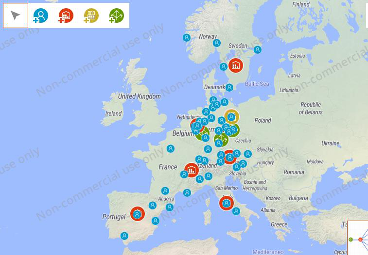
Figure 6: Alternative DCs locations
| Sites / costs in ($) |
|
||||
|---|---|---|---|---|---|
|
120 | 0.20 | 0.66 | 1.00 | 0.07 |
|
70 | 0.10 | 0.33 | 0.5 | 0.035 |
| 310 | 0.40 | 1.02 | 1.55 | 0.108 | |
| 120 | 0.20 | 0.68 | 1.07 | 0.07 | |
| 146 | 0.20 | 0.96 | 1.46 | 0.102 | |
| 90 | 0.20 | 0.33 | 0.5 | 0.05 | |
|
100 | 0.20 | 0.66 | 1.00 | 0.07 |
|
2,630 | 0.005 | 0.66 (beer) | 0.07 |
|
|---|
25
| Step 2. Analyze the results usingstatistics “Optimization Results”, “Flow Details”, “Produc- |
|---|
|
|---|
Given the threat of DC disruptions and the expansion plans with new customers, BERLIN BREWERY decides to redesign the SC by adding a second DC in Spain, which means that the fifth-best alternative is chosen out of 10 best SC designs displayed in “Optimization results”. The difference in profit between the best and the fifth-best SC design is very small but the SC design with 2 DCs offers more flexibility and resilience.
3.5 Simulation
- We introduce inventory control to manage ordering processes.
- We introduce sourcing policy (e.g., single vs. multiple sourcing) to manage replenish- ment processes
- We introduce shipment control (LTL/FTL) to manage shipment processes.
To evaluate the simulation results, we consider six KPIs according to the needs of BERLIN BREWERY:
(1)Financial KPIs, such as profit, revenue and costs
(2)Service level by products, which is calculated as (number of outgoing orders / number of placed orders), where an outgoing order is an order that is not dropped
(3)Available inventory including backlog at DCs.
| Step 2. Enter data from Table 4 in tables “Inventory”, “Sourcing”, “Paths”, and “Shipping”. |
|---|
|
|---|
b)Is demand for all customers satisfied? Explain.
c)What is your judgment on the inventory dynamics in the SC? Explain the change in inventory dynamics in the second part of the simulation period.
|
|---|
a)What are the profit, revenue, and costs of the SC for the two different network design scenarios?
b)Is demand for all customers satisfied? Explain.
|
|---|
|
|---|
3.8 Validation using Variation
Rather than running the same simulation multiple times with different parameter values or com-binations, the variation experiment allows multiple variations of the same simulation to be run simultaneously. A variation experiment highlights how KPIs change depending on different parameter values. This kind of sensitivity analysis can also be used to verify the validity of the results of the simulation model.
|
|---|
|
|---|
Develop recommendations for BERLIN BREWERY management. Consider GFA, NO, Simu-
lation, Comparison, and Variation results. Which SC design would you recommend? Consider
Berlin School of Economics and Law, 5th Edition
Ivanov, D., Tsipoulanidis, A., Schönberger, J. (2021): Global Supply Chain and Operations Management - A Decision-Oriented Introduction to the Creation of Value, Springer In- ternational Publishing Switzerland, 3rd Edition
Maak, K., Haves, J., Stracke, S. (2011) Entwicklung und Zukunft der Brauwirtschaft in Deutschland https://www.boeckler.de/pdf/p_edition_hbs_260.pdf (Dec 12, 2017) o.V .(2017) Unser Reinheitsgebot - Brauer Bund. http://www.brauer-bund.de/ (Nov 22, 2017) o.V. (2015) From Grains to Growlers: A Look at the Craft Beer Industry Supply Chain Mate- rial Handling and Logistics http://www.mhlnews.com/global-supply-chain/grains-growl- ers-look-craft-beer-industry-supply-chain-infographic (Dec 12, 2017)
o.V. (2016) Bierkonsum in Deutschland bis 2016 Statista. https://de.statista.com/statistik/da- ten/studie/4628/umfrage/entwicklung-des-bierverbrauchs-pro-kopf-in-deutschland-seit- 2000/ (Nov 12,2017)
Plank, R. (2013) Die Anwendung der Kälte in der Lebensmittelindustrie. Springer-Verlag, Heidelberg.
30