
And major health and milestone events are recorded
Continuous probability distributions
Continuous probability distributions – A guide for teachers (Years 11–12)
Published by Education Services Australia
PO Box 177
Carlton South Vic 3053
Australia
Tel: (03) 9207 9600
Fax: (03) 9910 9800
Email: info@esa.edu.au
Website: www.esa.edu.au

Probability density functions . . . . . . . . . . . . . . . . . . . . . . . . . . . . . . . 12
Mean and variance of a continuous random variable . . . . . . . . . . . . . . . . . 15
Continuous
probability
distributionsAssumed knowledge
The module Discrete probability distributions introduces the fundamentals of random variables, noting that they are the numerical outcome of a random procedure.
Most of the examples considered in that module involve counts of some sort: the number of things, or people, or occurrences, and so on. When we count, the outcome is definitely discrete: it can only take integer values, and not other numerical values.
Content
Continuous random variables: basic ideas
We have already seen examples of continuous random variables, when the idea of a ran-dom variable was first introduced.
|
|---|
|
Both discrete and continuous random variables have cdfs, although we did not focus on them in the modules on discrete random variables and they are more straightforward to use for continuous random variables.
As noted in the module Discrete probability distributions, the use of lower case x as the argument is arbitrary here: if we wrote FX (t), it would be the same function, determined by the random variable X . But it helps to associate the corresponding lower-case letter with the random variable we are considering.
=⇒ Pr(a < X ≤ b) = Pr(X ≤ b)−Pr(X ≤ a)
=⇒ Pr(a < X ≤ b) = FX (b)−FX (a).
All of the above discussion applies equally to discrete and continuous random variables.
We now turn specifically to the cdf of a continuous random variable. Its form is some-thing like that shown in the following figure. We require a continuous random variable to have a cdf that is a continuous function.
Figure 1: The general appearance of the cumulative distribution function of a continuous random variable.
We now use the cdf a continuous random variable to start to think about the question of probabilities for continuous random variables. For discrete random variables, probabil-ities come directly from the probability function pX (x): we identify the possible discrete values that the random variable X can take, and then specify somehow the probability for each of these values.
But what if we are interested in the probability that a continuous random variable takes a specific single value? What is Pr(X = x) for a continuous random variable?
We can address this question by considering the probability that X lies in an interval, and then shrinking the interval to a single point. Formally, for a continuous random variable X with cdf FX (x):
(since FX is continuous)
Hence, Pr(X = x) = 0. This is a somewhat disconcerting result: It seems to be saying that we can never really observe a continuous random variable taking a specific value, since the probability of observing any value is zero.
This is a discrete random variable, with the same probability for each of the ten possible outcomes.
Now suppose that instead we record X2, the random number truncated to two decimal places (again, not rounding). For example, if the real number is 0.9790295134, we record 0.97. This random variable is also discrete, with
| s o | f | 1 | 2 | r | e | s | i | |||||||||||||||||||||||||||||||||||||||||||||||||||||||||||||||||||||||||||||||||||||||||||||||||||||||
|---|---|---|---|---|---|---|---|---|---|---|---|---|---|---|---|---|---|---|---|---|---|---|---|---|---|---|---|---|---|---|---|---|---|---|---|---|---|---|---|---|---|---|---|---|---|---|---|---|---|---|---|---|---|---|---|---|---|---|---|---|---|---|---|---|---|---|---|---|---|---|---|---|---|---|---|---|---|---|---|---|---|---|---|---|---|---|---|---|---|---|---|---|---|---|---|---|---|---|---|---|---|---|---|---|---|---|---|---|---|---|
| 0.10 | ||||||||||||||||||||||||||||||||||||||||||||||||||||||||||||||||||||||||||||||||||||||||||||||||||||||||||||||
| 0.09 | ||||||||||||||||||||||||||||||||||||||||||||||||||||||||||||||||||||||||||||||||||||||||||||||||||||||||||||||
| 0.08 | ||||||||||||||||||||||||||||||||||||||||||||||||||||||||||||||||||||||||||||||||||||||||||||||||||||||||||||||
| 0.07 | ||||||||||||||||||||||||||||||||||||||||||||||||||||||||||||||||||||||||||||||||||||||||||||||||||||||||||||||
| 0.06 | ||||||||||||||||||||||||||||||||||||||||||||||||||||||||||||||||||||||||||||||||||||||||||||||||||||||||||||||
| 0.05 | ||||||||||||||||||||||||||||||||||||||||||||||||||||||||||||||||||||||||||||||||||||||||||||||||||||||||||||||
| 0.04 | ||||||||||||||||||||||||||||||||||||||||||||||||||||||||||||||||||||||||||||||||||||||||||||||||||||||||||||||
| 0.03 | ||||||||||||||||||||||||||||||||||||||||||||||||||||||||||||||||||||||||||||||||||||||||||||||||||||||||||||||
| 0.02 | ||||||||||||||||||||||||||||||||||||||||||||||||||||||||||||||||||||||||||||||||||||||||||||||||||||||||||||||
| 0.01 | ||||||||||||||||||||||||||||||||||||||||||||||||||||||||||||||||||||||||||||||||||||||||||||||||||||||||||||||
0.00 Pr ��� � �� |
0. | 0 | 0 | . | 1 | 0 | . | 2 | 0 | . | 3 | 0 | . |
|
||||||||||||||||||||||||||||||||||||||||||||||||||||||||||||||||||||||||||||||||||||||||||||||||
| 0.10 | ||||||||||||||||||||||||||||||||||||||||||||||||||||||||||||||||||||||||||||||||||||||||||||||||||||||||||||||
| 0.09 | ||||||||||||||||||||||||||||||||||||||||||||||||||||||||||||||||||||||||||||||||||||||||||||||||||||||||||||||
| 0.08 | ||||||||||||||||||||||||||||||||||||||||||||||||||||||||||||||||||||||||||||||||||||||||||||||||||||||||||||||
| 0.07 | ||||||||||||||||||||||||||||||||||||||||||||||||||||||||||||||||||||||||||||||||||||||||||||||||||||||||||||||
| 0.06 | ||||||||||||||||||||||||||||||||||||||||||||||||||||||||||||||||||||||||||||||||||||||||||||||||||||||||||||||
| 0.05 | ||||||||||||||||||||||||||||||||||||||||||||||||||||||||||||||||||||||||||||||||||||||||||||||||||||||||||||||
| 0.04 | ||||||||||||||||||||||||||||||||||||||||||||||||||||||||||||||||||||||||||||||||||||||||||||||||||||||||||||||
| 0.03 | ||||||||||||||||||||||||||||||||||||||||||||||||||||||||||||||||||||||||||||||||||||||||||||||||||||||||||||||
| 0.02 | ||||||||||||||||||||||||||||||||||||||||||||||||||||||||||||||||||||||||||||||||||||||||||||||||||||||||||||||
| 0.01 | ||||||||||||||||||||||||||||||||||||||||||||||||||||||||||||||||||||||||||||||||||||||||||||||||||||||||||||||
|
tio : A |
o e |
i i t |
s x |
i a |
t e |
1 g |
p o s t |
r r |
t e |
o |
r e |
0 a |
u d |
2 | s |
l |
l l |
l e |
r t e |
f |
. |
3 r |
l o u i |
t t |
o t |
r | 0 n |
. t |
s pX1(x) for X1 and pX2(x) for X2. the frst k decimal places, the random vari-h the same probability 10−k. |
||||||||||||||||||||||||||||||||||||||||||||||||||||||||||||||||||||||||||||||||
Now consider the chance that each of these discrete random variables X1,X2,X3,... takes a value in the interval [0.3,0.4), for example. We have
Pr(0.3 ≤ X1 < 0.4) = Pr(X1 = 0.3) = 0.1,
As k increases, the discrete random variable Xk can be thought of as a closer and closer approximation to a continuous random variable. This continuous random variable, which we label U, has the property that
Pr(a ≤U ≤ b) = b − a, for 0 ≤ a ≤ b ≤ 1.

A guide for teachers – Years 11 and 12 • {11}
0.6
0.4
| 0.0 | 0.2 | 0.4 | 0.6 | 0.8 | |
|---|---|---|---|---|---|
|
|||||
You might have noticed a difference in how the interval between 0.3 and 0.4 was treated in the continuous case, compared to the discrete cases. In all of the discrete cases, the upper limits 0.4,0.40,0.400,... were excluded, while for the continuous random variable it is included. Whenever we are dealing with discrete random variables, whether the inequality is strict or not often matters, and care is needed. For example,
{12} • Continuous probability distributions
Probability density functions
| F(x) = | �x−∞ |
|
|---|
The pdf f (x) has two important properties:
We now explore how probabilities concerning the continuous random variable X relate to its pdf. The important result here is that
|
�b | f (x) dx = |
|---|
• For a continuous random variable, we must consider the probability that it lies in an interval. The importance of this result is that it tells us that, to find the probability, we need to find the area under the pdf on the given interval.
• The total area under the pdf equals 1. So this result tells us that, to approximate the probability that the random variable lies in a given interval, we just have to guess the fraction of the area under the pdf between the ends of the interval.
a Check that f (x) has the two required properties for a pdf, and sketch its graph. f (x) = 6x(1− x) 0 if 0 ≤ x ≤ 1, otherwise.
b Suppose that the continuous random variable X has the pdf f (x). Obtain the follow- ing probabilities without calculation:
A guide for teachers – Years 11 and 12 • {15}
e Which is more likely: V ≈ 0.3 or V ≈ 0.8? Explain.
The triangular pdf shown in figure 7 is the pdf of the average of two U(0,1) random vari-
| ables. That is, if U1 | d= U(0,1) and U2 | |
|---|---|---|
| the pdf in figure 7. |
�����
Mean and variance of a continuous random variable
Mean of a continuous random variable
probability function pX (x) is
|
|---|
The equivalent quantity for a continuous random variable, not surprisingly, involves an integral rather than a sum. The mean µX of a continuous random variable X with prob-ability density function fX (x) is
Exercise 3
Two triangular pdfs are shown in figure 9.
0.00 0.20 |
|||||
|---|---|---|---|---|---|
| 0 |
|
4 | 6 | 10 | |
| 0 | 3 | 4 | 7 | 10 | |
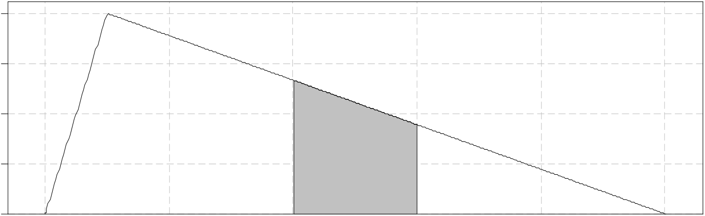
boundaries of the shaded region are labelled on the x-axis in figure 9.
For each of these pdfs separately:
The module Discrete probability distributions gives formulas for the mean and variance
of a linear transformation of a discrete random variable. In this module, we will prove
for any real numbers a,b.
Proof
var(X ) = σ2 X= E[(X −µ)2], where µ = E(X ).
The variance of a continuous random variable X is the weighted average of the squared deviations from the mean µ, where the weights are given by the probability density func-tion fX (x) of X . Hence, for a continuous random variable X with mean µX , the variance of X is given by
| var(X ) = σ2 X= E[(X −µX )2] = | �∞−∞ |
|---|
a the random variable U d= U(0,1); see figure 6
b the random variable V from exercise 2.As observed in the module Discrete probability distributions, there is no simple, direct interpretation of the variance or the standard deviation. (The variance is equivalent to the ‘moment of inertia’ in physics.) However, there is a useful guide for the standard deviation that works most of the time in practice. This guide or ‘rule of thumb’ says that, for many distributions, the probability that an observation is within two standard deviations of the mean is approximately 0.95. That is,
For the random variable V from exercises 2 and 4, find Pr(µV −2σV ≤ V ≤ µV +2σV ).
A guide for teachers – Years 11 and 12 • {19}
Proof
Define Y = aX +b. Then var(Y ) = E[(Y −µY )2]. We know that µY = aµX +b. Hence,var(aX +b) = E��aX +b −(aµX +b)�2�
= E�a2(X −µX )2�
= a2E[(X −µX )2]
= a2var(X )
| = a2σ2 X. |
|---|
Relative frequencies and continuous distributions
Continuous random variables are technically an abstraction (Pr(X = x) = 0), and all vari-ables that we measure are in practice, as measured, discrete. Even quantities that seem to be intrinsically continuous, like time, are always measured to the nearest unit of time, depending on the context. The following table illustrates this.
The answer is that it is often convenient and useful to use a continuous distribution, rather than attempting to use a discrete model.
Example: Train trips
|
Frequency | Relative frequency |
|
|---|---|---|---|
| 41:00 – 41:59 | 87 | 0.348 | 0.345 |
| 42:00 – 42:59 | 68 | 0.272 | 0.271 |
| 43:00 – 43:59 | 38 | 0.152 | 0.142 |
| 44:00 – 44:59 | 22 | 0.088 | 0.081 |
| 45:00 – 45:59 | 9 | 0.036 | 0.049 |
A guide for teachers – Years 11 and 12 • {23} Answers to exercises
| �∞−∞ | f (x) dx = | �1 | |
|---|---|---|---|
| = | �1 | ||
|
|||
| b |
|
|
|---|---|---|
| i |
|
|
= 0.432.
| d | i |
|
|||
|---|---|---|---|---|---|
| ii | p0.2 = Pr(0.15 ≤ X ≤ 0.25) = | �0.25 | |||
| iii | |||||
| p0.4 = Pr(0.35 ≤ X ≤ 0.45) = | �0.45 | ||||
| iv | p0.4 | ||||
| p0.2 | |||||
| c | For v > 0, we have FV (v) =�v fV (t) dt. We need to deal with the two parts of the pdf
|
|---|
=1 2+(4v −2v2)−
3
= 4v −2v2−1.Putting these two parts together, we can write, formally, that the cdf of V is given by
| a | |||
|---|---|---|---|
45(10− x) 1 |
|||
| f (y) = |
|
||
b You need to guess where the centre of gravity of the pdf is, that is, where you would
need to put the pivot to make the pdf balance. Reasonable guesses would be ‘be-
| c | E(Y ) = | �∞−∞ | ||||||||
|---|---|---|---|---|---|---|---|---|---|---|
| = |
|
|||||||||
| = | ||||||||||
| = | �64 60−0� | +1 30 | ��500−1000 | � | − | �80−64 | ||||
|
||||||||||
otherwise.
2.
Exercise 5
From the previous exercise, we have µV = 0.5 and σV = 0.204. Thus
Pr(0.5−0.408 ≤ V ≤ 0.5) = Pr(0.092 ≤ V ≤ 0.5)
=�0.5 0.092
Hence, Pr
probability 0.95 indicated by the rule of thumb.�µV −2σV ≤ V ≤ µV +2σV�= 2×0.483 = 0.966. This is reasonably close to the
Recall that sd(aX + b) = |a|sd(X ). Since sd(X ) = 50, this gives sd(Y ) = 2.20 × 50 = 110.
The standard deviation of the cost is $110.
| 0 | 1 | 2 | 3 | 4 | 5 | 6 | 7 | 8 | 9 | 10 | 11 |
|---|