Check the error the results part applying equation

Today’s lab consists of four parts:

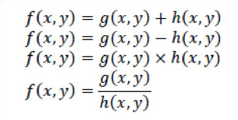
1.First, you will learn about some basic image arithmetic operations.

ignal. Some basic arithmetic operations from the text are as follows:

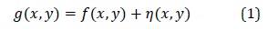
Consider an image 𝑓𝑓(𝑥𝑥,𝑦𝑦). When 𝑓𝑓(𝑥𝑥,𝑦𝑦) is captured it is corrupted by noise. Perhaps the photographer had a very high ISO value or some other factor. Let 𝑔𝑔(𝑥𝑥,𝑦𝑦) be the image which was captured and saved in a digital format. Let us assume that the noise 𝜂𝜂(𝑥𝑥,𝑦𝑦) is additive:

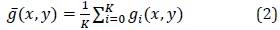
You may be asking yourself, just how effective is Equation 2 anyway? This is an important question to ask, and we must come up with some way to measure how well it works. This is important because it can be used to compare different methods for your project. The problem is this: we must compare the difference between 𝑔𝑔̅(𝑥𝑥,𝑦𝑦) and 𝑓𝑓(𝑥𝑥,𝑦𝑦). Because 𝑓𝑓(𝑥𝑥,𝑦𝑦) is the original image we used to create the artificial, noisy data, if we did a good job with Equation (2), 𝑔𝑔̅(𝑥𝑥,𝑦𝑦) should be similar to 𝑓𝑓(𝑥𝑥,𝑦𝑦). One way to carry out this comparison is by computing the city-block distance of each pixel and taking the average. This will give you a rough estimate of how much error is occurring amongst all the pixels:

In this part of the lab, you will download the image from Canvas and corrupt it with normally distributed noise. This image was selected because of it has large contiguous areas with the same tone (you can easily see the noise). Load it with imread. This image will be 𝑓𝑓(𝑥𝑥,𝑦𝑦). Generate some noisy samples of 𝑓𝑓(𝑥𝑥,𝑦𝑦) by carrying out Equation (1), restated here:

function g = corruptImage( f )
[m n] = size( f ); g =
zeros( size( f ) ); for
i = 1:m for j =
1:n
< YOUR CODE HERE >
end end

Note that it’s possible to use randn in a more elegant way. Type help randn to find out more.

= corruptImage( f )

And view it with:

Show both images at the same use the subplot figure generator:

subplot(1,2,1), imshow( g1, [0 255] ); subplot(1,2,2), imshow( f – g1, [0 255] );

Now that we have generated our artificially noisy data, we can estimate the original image using Equation 2, restated here:

Looking at the result in Part 2 was subjective, and we can use Equation (3) to come up with an objective measurement. Check the error of the results in part 2 by applying Equation (3). Create your own function called MAD to apply equation 3. It should take two images as an input and output a single value.

Vary the number of averages you do in part 2 from 2 to 100 and plot the MAD values. Use plot in MATLAB to visualize your experiment. This should all be in one script.

Additional Questions

5.Define a Normal Distribution and describe its parameters.