Clicking the powerpivot tab displays the options shown figure png

How do I read data into PowerPivot?

How do I use PowerPivot to create a PivotTable?

Answers to This Chapter’s Questions: How do I read data into PowerPivot?

After you install PowerPivot, you see a PowerPivot tab on the ribbon. Clicking the PowerPivot tab displays the options shown in Figure 84-1.

Figure 84-2. The PowerPivot window Home tab.

If you installed PowerPivot after October 2010, you will also see an option for getting external data from the Windows Azure Datamarket. This option enables you to conduct PowerPivot analyses on a variety of interesting data sets described at datamarket.azure.com. For example, you can download game-by-game statistics from all NFL games and break down how each team performed rushing and passing against teams in its own division.

After copying data from Excel, you can select Paste to insert the data into PowerPivot.

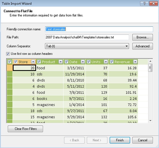
To illustrate how to download data from multiple sources into PowerPivot, I’ll use the text file Storesales.txt, in which I’ve listed sales transactions from 20 stores. A subset of the data is shown in Figure 84-3. You can see that for each transaction, I am given the store number, the product sold, sale date, units sold, and revenue. I want to summarize this data by state, but the state for each store is listed in a different file, States.xlsx. The location of each store is shown in Figure 84-4.

I want to create a PivotTable that lets me slice and dice my data so that I can view how I did selling each product in each state. To begin, I select the PowerPivot tab and then click PowerPivot Window in the Launch group (as shown at the left in Figure 84-1). This brings up the Home tab in the PowerPivot window. Because I want to import a text file, I select From Text on the Home tab. As shown in Figure 84-5, I can then browse to the file Storesales.txt. Because the first row of data contains column headers, I select the Use First Row As Column Headers option. In the Column Separator list, I select Tab because the data fields in the text file are not separated by spaces or a character, such as a comma or a semicolon. Clicking Finish imports the text file’s data into PowerPivot.

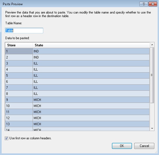
$C:\Users\AKamel\AppData\Local\Temp\httpatomoreillycomsourcemspimages1576606.png.jpg$

Next, I want to import the file States.xlsx so that PowerPivot will know the state in which each store is located. To import States.xlsx, I return to Excel by clicking the Excel icon in the upper-left corner of the PowerPivot ribbon. Then I open the file States.xlsx and copy the data I need. Now, I select Paste on the Home tab in PowerPivot (see Figure 84-2). The Paste Preview dialog box shown in Figure 84-7 appears.

$C:\Users\AKamel\AppData\Local\Temp\httpatomoreillycomsourcemspimages1576610.png.jpg$

Recall that I want to analyze sales in different states. The problem is that at present PowerPivot does not know that the listing of store locations from States.xlsx corresponds to the stores listed in the text file. To remedy this problem, I need to create a relationship between the two data sources. To create this relationship, I click Design on the ribbon in the PowerPivot window (see Figure 84-2) to display the Design tab shown in Figure 84-9.

PowerPivot Design tab.

Figure 84-10. Creating a relationship between two data sources.

How do I use PowerPivot to create a PivotTable?

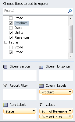
$C:\Users\AKamel\AppData\Local\Temp\httpatomoreillycomsourcemspimages1576620.png$

Figure 84-12. Assignment of fields to create a PivotTable report.

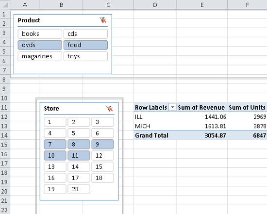
In Chapter 43, I showed how to use slicers to reveal details and different perspectives in your PivotTable analyses. Slicers look even nicer in PowerPivot PivotTables. Here, I’ll create slicers that summarize the data for any subset of products and stores. To do this, I place Product in the Slicers Horizontal field area and Store in the Slicers Vertical area in the PowerPivot Field List. The resulting slicers are shown in Figure 84-14. (See the file Pivotwithslicers.xlsx.) As described in Chapter 43, you can hold down the Ctrl key as you click to select any subset of products and/or stores. Holding down the Ctrl key also enables you to resize the slicers. The PivotTable shown in Figure 84-14 gives the total revenue and units sold of DVDs and food in Stores 7 through 11. Since Stores 7 through 11 are all in Illinois or Michigan, these are the only states shown in the resulting PivotTable. If I had created the Product slicer with the ordinary Excel PivotTable functionality, all six products would be listed in a single column. I think you would agree that the PowerPivot Product slicer looks much nicer.

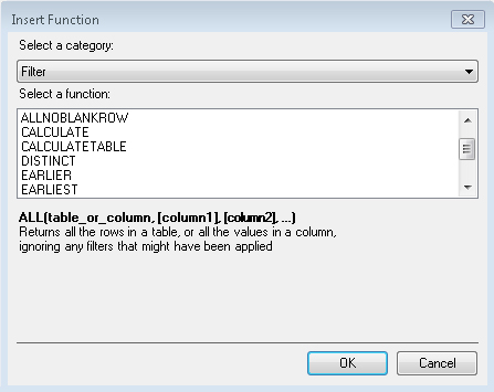
$C:\Users\AKamel\AppData\Local\Temp\httpatomoreillycomsourcemspimages1576624.png.jpg$

To illustrate a DAX formula, I’ll show how to place the year, month, and day of the month for each sales transaction in a separate column. To begin, I click the Storessales tab in the PowerPivot window and select the first blank column. Clicking the fx button below the PowerPivot ribbon brings up a list of DAX functions. Many of these (such as YEAR, MONTH, and DAY) are virtually identical to ordinary Excel functions. Selecting Filter brings up the list of DAX functions shown in Figure 84-15. These are not your mother’s Excel functions! For example, the DISTINCT function can return a list of entries in a column that meet a specified criterion.

$C:\Users\AKamel\AppData\Local\Temp\httpatomoreillycomsourcemspimages1576626.png$

Now I can create a variety of informative PivotTables. For example, I can summarize sales in each state by year. (See Problem 1.)

Problems

P1: Summarize total sales in each state by year.

P2: Summarize total revenue by store and create a slicer for stores.

Q4.What are DAX functions?

All submissions should include detailed excel work, with all outputs, and outcomes, as well as be submitted in APA format if a written part is required to explain results. All excel sheets and workbook(s) must be submitted, Excel pdf, and copy.past excel as picture into documents is not accepted.

Header with assignment title and page number.
Page margins Top, Bottom, Left Side and Right Side = 1 inch, with reasonable accommodation being made for special situations and online submission variances.