
Modeling and processing decision support queries
Columbia University
Abstract
1.1. Ad hoc OLAP Queries
Although significant research has been conducted on datacubes [12], both in terms of modeling [2] and evalua-tion [1, 17], little has been done on query optimization of complex ad hoc decision support queries, despite of their importance. To express such queries in SQL, a high degree of redundancy is required: multiple self-joins, correlated subqueries and repeated group-bys. This leads to compli-cated queries, difficult to understand and optimize. Stan-dard query processing techniques [8, 22] help somehow. The problem is that a traditional SQL optimizer will not consider the “big picture”, but will try to optimize a series of joins and aggregations, which is not always the best approach. In [7] we have addressed this issue and provided techniques to combine joins and aggregations into a more general operation. Similar concerns are discussed in [23]. However, there are many important queries that do not fall in this framework. Consider some typical OLAP queries over the following relation:
product and sales of 1997, show the product’s average sale before and after each month of 1997.” (trends)
Standard SQL representations of these queries require several views joined together or correlated subqueries. These complex representations lack succinctness, a nec-essary aspect for efficient optimization. For example, Query Q1 could be expressed in standard SQL with a 3-way self-join2 (views could be used as well) :
select x.product, sum(x.quantity), sum(y.quantity), sum(z.quantity)
To have a row for every product in the answer, joins must be replaced by outer-joins since some products may have NULL values for January, February, or March.
1.2. Syntax : Looping is Important
t.product=p and t.month<m;
avg_y = avg(t), where tuples t have t.product=p and t.month>m;
Traditionally, an SQL query translates to a relational algebra expression and the query processor optimizes this expression. A complex query may involve several join and aggregation operators. The job of the optimizer is to commute operators in an equivalent and optimal way, and choose appropriate algorithms for each operator [9]. Con-sider once again Query Q2. One possible SQL formulation is presented below.
|
|||
| ing to the (p m ) value. | |||
where x.product=y.product and x.month > y.month
group by x.product, x.month
where B1.product=B2.product and B1.month=B2.month
Traditional systems would try to formulate for each (p m )
Syntax A syntactic extension of SQL that can express most ad hoc decision support queries concisely and succinctly is introduced. This allows the user to write, understand and maintain complex OLAP queries sig-nificantly easier (although SQL’s expressive power is not extended.)
Evaluation Evaluation of queries expressed with our syn-tactic construct maps directly to an efficient evaluation
In [6] we have introduced the concept of multi-feature queries which has proven useful for certain OLAP and datacube queries[18]. In this section we extend slightly this syntax, covering however a significantly larger class of data analysis queries. These queries are called extended multi-feature queries (EMF queries.)
2.1. Multi-Feature Syntax
group by product : X, Y, Z such that X.month = 1,
Y.month = 2,
ables. These are declared in the group by clause as be-fore, separated by the grouping attributes with a semicolon. However, the scope of these grouping variables is not any longer the group, but the entire relation. The assumption that grouping variables are subsets of the group is dropped. As a result, the defining conditions of the grouping variables may involve one or more of the grouping attributes, which can be considered as constants for the currently processed group 4. Formally, the syntactic extensions are:
Each Ci is a (potentially complex) condition that is
used to define Xi grouping variable, i = 1 2 . It may involve (i) attributes of Xi, (ii) constants, (iii) grouping attributes, (iv) aggregates of the group and
Definition 2.1: The output of a grouping variable X, de-noted as outp(X), is the set of the aggregates of X that ap-pear either in the such that clause, the select clause, or the having clause. 2
The grouping attributes have a unique value within a group. As a result, grouping attributes can be considered as constants for the such that clause, similar to the aggregates of the group. This is why we can extend multi-feature syntax. Otherwise the such that conditions would not be able to translate to simple selections over the relation. Rather, they would express joins.
where year=‘‘1997’’
group by product, month; X , Y such that X.product=product and
Query Q3 exhibits two levels of aggregation, i.e. ag-gregated values at a first level are used at a second level of aggregation, something common in data mining queries. This can be expressed easily with the EMF syntax, due to the succesive declaration of grouping variables.
select product,month,count(X.*),count(Y.*) from Sales
select product, month, year, sum(X.quantity)/sum(Y.quantity)
from Sales
This query can be expressed using just Y grouping variable. Since X represents the entire group, sum(X.quantity) could be replaced by sum(quantity).
of the group and the grouping variables. Then we take the projection over the join of these 2n + 1 relations according to the attributes in the select clause. Formally, the semantics in relational algebra are defined as follows.
Definition 2.2: Assume that S is the set of the grouping attributes, D is the domain of the grouping attributes, Xi,
| 1. For each value x 2 D, define: | |||||||
|---|---|---|---|---|---|---|---|
|
|||||||
| 0 | |||||||
|
|||||||
| Ci | |||||||
| i | 0 |
|
|||||
|
|||||||
2. The result is given by:
S s(F x 1 : : : 1 F x 1 Xx 1 : : : 1 Xx), where
Note that the result may have many duplicate rows due to the join in the last step of Definition 2.2. This topic is discussed in length in [6]. One solution to this problem is to get the join only of the grouping variables (Xix’s) and/or the aggregates (Fix’s) mentioned in the select clause.
Another issue concerns empty grouping variables. Ac-cording to the previous definition, if a grouping variable of
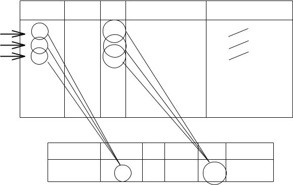
Example 3.1: Consider Example 2.2 and Query Q4. The mf-structure H of this query, corresponding roughly to its output schema, is given in Figure 1(a). Initially, the algo-rithm scans the Sales relation to complete the product, month, year columns, i.e. to find the distinct values of the grouping attributes (Figure 1(b).) During the sec-ond scan of Sales, the algorithm computes the aggregate sum(X.quantity) of the first grouping variable X, by identifying for each tuple t of Sales relation the rows of
that satisfy X’s defining condition in the such that clause with respect to t, and update them appropriately. Figure 1(c) shows a currently scanned tuple t, the row of
Product Month Year sum(X.Quantity) sum(Y.Quantity)
(b) end of first scan
| H : | Product Month Year sum(X.Quantity) sum(Y.Quantity) | ||||||
|---|---|---|---|---|---|---|---|
| 1 | 1997 | 216 | |||||
| 2 | 1997 | 122 | 269 | ||||
| 5 | 1997 | 245 | |||||
|
2 | 1997 | 455 | ||||
|
3 | 1997 | 196 | ||||
| 6 | 1997 | 386 | |||||
| 9 | 1997 | 265 | |||||
| H : |
|
|||||
|---|---|---|---|---|---|---|
| 1 | 1997 | 241 | 265 | |||
| 2 | 1997 | 241 | 265 | |||
|
5 | 1997 |
|
241 | 265 | |
| 2 | 1997 | 411 | ||||
| 3 | 1997 | 411 | ||||
|
6 | 1997 |
|
411 | ||
| 9 | 1997 | 411 | ||||
Figure 1. Several phases of evaluation of Query Q4
Definition 3.1: Let Q be an extended multi-feature query and H be a table with columns the grouping attributes and the output of each grouping variable (outp(Xi), i =
for scan sc=0 to n f
for each tuple t on scan sc f
priately.X0 denotes the group (the
defining condition of X0 is X0:S = S,
may belong to grouping variable Xi of several groups, as in Query Q4 : a tuple t affects several groups with respect to grouping variable Y , namely those that agree on product,year with t’s product, year.
The only access method used in our algorithm is scan-ning (or indexed scanning). As a result, the evaluation of multiple EMF queries can overlap since the query-specific computation takes place in the individual mf-structure.
Algorithm 3.1 can become very expensive if the mf-structure has a large number of entries since, for every scanned tuple all H’s entries are examined, resulting in an implicit nested-loop join. However, this is not always necessary since, given a tuple t, one can identify a small number of mf-structure’s entries that may be updated w.r.t t during the evaluation of a grouping variable X.
Example 4.1: Consider Query Q4. During the evaluation of grouping variable X (scan 1) and a tuple t, only one entry of Q4’s mf-structure H is updated, the one that agrees on product, month and year with t. This is not the case during the evaluation of grouping variable Y (scan 2). For a scanned tuple t there is a set of H’s entries that are updated, namely those that agree on product, year with t.
Although we may not know precisely the contents of Rel(X t ) w.r.t. a grouping variable X and a tuple t, we may be able to determine what entries will not be included in Rel(X,t). This limits the search for relative entries within a small subset of the mf-structure, reducing the overall cost significantly. By recognizing this fact, we can keep H as a special data structure that makes searching fast (e.g. a hash table or a B+-tree), in order to locate the relative entries fast. For example, the mf-structure of Query Q4 can be kept as
a hash table on product, year using a hash function h. Given a tuple t one searches only the entries stored in bucket h(t:product t:year ). Our prototype implemen-tation (described in Section 5) assumes conjunctive such that clauses and uses a simple algorithm that checks syntactically the such that clauses to determine if the mf-structure of a query can be kept as a hash table on some subset of the grouping attributes.
Definition 4.2: If a grouping variable Y contains in its such that clause one or more aggregates of another grouping variable X, then we say that Y depends on X and we write Y ! X. If Y ’s such that clause mentions one or more of the grouping attributes, then we say that Y depends on X0 and we write Y ! X0. The directed acyclic graph formed by the grouping variables’ interdependencies of an EMF query is called the emf-dependency graph of the query. 2
One can analyze syntactically the such that clauses of a query and create its emf-dependency graph G. We can find the minimal number of required scans and the grouping variables computed on each scan by sorting topologically graph G. There are cases however that this minimal number can be further reduced by evaluating two or more dependent grouping variables in the same scan in the event of some additional knowledge.
A set of similar optimizations in the context of tape-resident data warehouses and temporal EMF queries appear in [4]. We are currently investigating additional cases of dependent grouping variables that can be evaluated in the same scan.
One can think of the optimizations of this section as a form of multiple query analysis [21]. In standard SQL, grouping variables would correspond to individual query blocks (if views were used) and a standard query processor would evaluate them independently, one after the other. We could say that multiple query analysis in extended multi-feature queries reduces to dependency analysis.
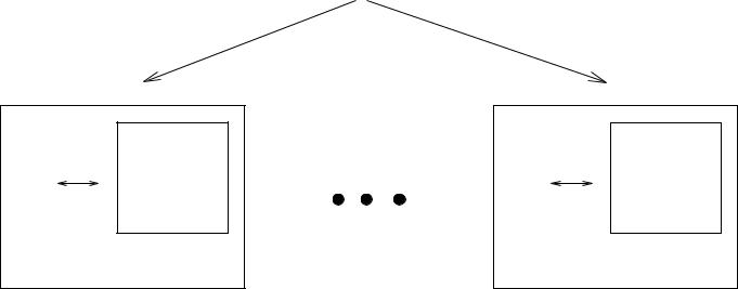
Reducing the cost of the mf-structure’s search is only one of the benefits of this optimization. It may be the case that the mf-structure of a query is too large to fit in one system’s memory. With this technique the mf-structure can be partitioned to fit to several systems’ memory in a clean, transparent way with no communication costs among the nodes.
4.4. More Scans, Less Memory
| t |
|
||
|---|---|---|---|
|
|
“rounds” instead of one, using only one node. During each “round”, only part of the mf-structure is computed by Algorithm 3.1.
This technique is conceptually the same to the method of the previous section, but it does not assume the presence of
on all these entries will be the same, the total quantity of t’s product on t’s year. It seems that we repeat the computation of a product’s yearly sum twelve times. One could decorrelate the computation of this grouping variable by creating a separate mf-structure.
However, the benefits of this optimization have to be assessed carefully for several reasons. The main idea is not as simple as before and Algorithm 3.1 has to change in
Below we compare the performance of the SQL compo-nent of the commercial database system versus our system’s performance on Queries Q1 and Q2. Similar results hold for Queries Q3, to Q6 7. During the experiments we were the only users of the system. Time measurements are elapsed times and each measurement is the average of several runs. The goal is not to prove that our system is bet-ter than some commerical DBMS(s), but to emphasize that traditional optimizers do not consider the special structure of extended multi-feature queries.
The performance of Query Q1 is shown in figure 3. The size of each group is 6 tuples. Our implementation gener-ates a program that computes the answer in one scan. The mf-structure is represented as a hash table on product. “SQL-A” and “SQL-B” correspond to two different stan-dard SQL representations (views, self-joins) of Query Q1, evaluated by the SQL component of the DBMS. The per-formance of our system is marked as “Implementation”. Our method uses the procedural language of the DBMS and this incurs a huge overhead in terms of scanning and processing. The line marked “Flat Files” shows what the performance of our method would be if Algorithm 3.1 has been implemented in the server, instead of on top of it. In order to get this measurement we used a different version of our implementation, operating on flat files and generating C programs incorporating Algorithm 3.1. Description and usage of this implementation appears in [3].
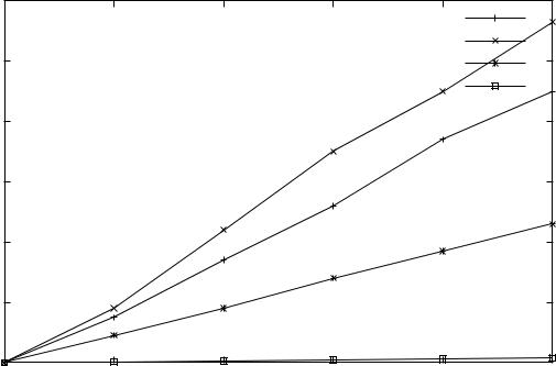
Size (number of groups)
| 180 | Standard SQL - A | ||||||
|---|---|---|---|---|---|---|---|
| 160 | Implementation | ||||||
| Flat Files | |||||||
| 140 | |||||||
| 120 | |||||||
| 100 | |||||||
| 80 | |||||||
| 60 | |||||||
| 40 | |||||||
| 20 | |||||||
| 0 | |||||||
| 0 | 1000 | 2000 | 3000 | 4000 | 5000 | ||
Size (number of groups)
Figure 4. Performance of Query Q2 using standard SQL vs EMF
expressed with standard SQL. We propose a simple and intuitive syntactic extension of SQL in order to express EMF queries. It equips SQL with a looping construct in a declarative way. We argue that such an extension is imperative to express and evaluate ad hoc OLAP queries. A simple evaluation algorithm and several optimizations are presented, showing the flexibility of our implementation.
D. Chatziantoniou. Introducing the PanQ Tool for Com-plex Data Management. In ACM International Conference on Knowledge Discovery and Data Mining (SIGKDD) (to appear), 1999.
D. Chatziantoniou and T. Johnson. Decision Support Queries on a Tape-Resident Data Warehouse. IEEE Com-puter (to appear).
D. DeWitt, S. Ghandeharizadeh, D. Schneider, A. Bricker, H. Hsiao, and R. Rasmussen. The Gamma Database Ma-chine Project. TKDE, 2(1):44–62, 1990.
R. Elmasri and S. Navathe. Fundamentals of Database Systems. The Benjamin/Cummings Publishing Company, 1989.
R. Meo, G. Psaila, and S. Ceri. A Tightly-Coupled Archi-tecture for Data Mining. In IEEE International Conference on Data Engineering, pages 316–323, 1998.
C. Red Brick Systems, Los Gatos. RISQL Reference Guide, Red Brick Warehouse VPT Version 3. 1994.
T. Sellis. Multiple-query Optimization. ACM Transactions on Database Systems, 13(1):23–52, 1988.
P. Seshadri, H. Pirahesh, and T. C. Leung. Complex Query Decorrelation. In International Conference on Data Engi-neering, pages 450–458, 1996.