
Table and figure for the standard gpt- model architecture
combined. However, combining these techniques leads to non-trivial interactions, which need to be reasoned through carefully for good performance. In this paper, we address the following question:
Achieving this throughput at scale required innovation and care-ful engineering along multiple axes: efficient kernel implementa-tions that allowed most of the computation to be compute-bound as opposed to memory-bound, smart partitioning of computation graphs over the devices to reduce the number of bytes sent over net-work links while also limiting device idle periods, domain-specific communication optimization, and fast hardware (state-of-the-art GPUs and high-bandwidth links between GPUs on the same and different servers). We are hopeful that our open-sourced software (available at ) will enable other groups scale.
In addition, we studied the interaction between the various com-ponents affecting throughput, both empirically and analytically when possible. Based on these studies, we offer the following guid-ing principles on how to configure distributed training:
2 MODES OF PARALLELISM
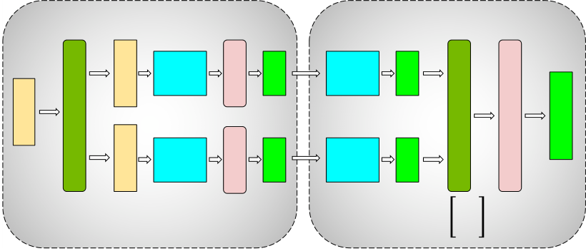
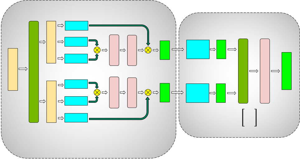
In this section, we discuss the parallelism techniques that facilitate the efficient training of large models that do not fit in the memory of a single GPU. In this work, we combine pipeline model parallelism and tensor model parallelism (combination shown in Figure 2) with data parallelism. We call this PTD-P for short.
A batch is split into smaller microbatches; execution is then pipelined across microbatches. Pipelining schemes need to ensure that inputs see consistent weight versions across forward and back-ward passes for well-defined synchronous weight update semantics. Specifically, naive pipelining can lead to an input seeing weight updates in the backward pass not seen in the forward pass.
To retain strict optimizer semantics exactly, we introduce peri-odic pipeline flushes so that optimizer steps are synchronized across devices. At the start and end of every batch, devices are idle. We call this idle time the pipeline bubble, and want to make it as small as possible. Asynchronous and bounded-staleness approaches such as PipeMare, PipeDream, and PipeDream-2BW [23, 29, 30, 45] do
Tensor MP partition #2 Tensor MP partition #2
Pipeline MP partition #1 Pipeline MP partition #2
| Device 1 | 7 1 8 2 5 3 6 4 7 1 8 2 | 3 | 4 | 5 | 6 | 7 | 8 | 5 | 6 | 7 | 8 9 1 0 | 1 | 29 1 | 1 | 1 | 1 |
|
|||||
|---|---|---|---|---|---|---|---|---|---|---|---|---|---|---|---|---|---|---|---|---|---|---|
| 1 | 1 | 2 | 3 |
|
||||||||||||||||||
| Device 2 | 5 | 6 | 7 | 8 | 5 | 6 | 7 | 8 | ||||||||||||||
| 9 1 0 | 1 | 29 1 | 1 | |||||||||||||||||||
| 1 | 1 |
|
||||||||||||||||||||
| Device 3 | 1 2 3 4 1 2 | 3 1 4 2 5 3 6 4 7 1 8 2 5 3 6 4 7 5 8 6 | 7 | 8 | 5 | 6 | 7 | 8 | ||||||||||||||
|
1 | 29 1 | ||||||||||||||||||||
| 1 | ||||||||||||||||||||||
| Device 4 | 5 | 6 | 7 | 8 | 9 1 0 | 1 | ||||||||||||||||
| 1 | ||||||||||||||||||||||
There are several possible ways of scheduling forward and back-ward microbatches across devices; each approach offers different tradeoffs between pipeline bubble size, communication, and mem-ory footprint. We discuss two such approaches in this section.
2.2.1 Default Schedule. GPipe [20] proposes a schedule where the forward passes for all microbatches in a batch are first executed,
| 𝑡𝑝𝑏 | =𝑝 − 1 | |||||
| 𝑡𝑖𝑑 | 𝑚 | |||||
|
||||||
| Bubble time fraction (pipeline bubble size) = | 𝑡int. 𝑝𝑏 | =1 𝑣· 𝑝 − 1 |
|
|||
| 𝑡𝑖𝑑 | ||||||
The MLP block consists of two GEMMs and a GeLU non-linearity:
𝑌 = GeLU(𝑋𝐴). 𝑍 = Dropout(𝑌𝐵).
The output of the second GEMM is then reduced across the GPUs before the dropout layer.
We exploit the inherent parallelism in the multi-head attention operation to partition the self-attention block (shown in Figure 5b). The key (𝐾), query (𝑄), and value (𝑉 ) matrices can be partitioned in a column-parallel fashion. The output linear layer can then directly operate on the partitioned output of the attention operation (weight matrix partitioned across rows).
Efficient Large-Scale Language Model Training on GPU Clusters Using Megatron-LM
| 𝑋 | 𝑋 | 𝑌! | 𝑌!𝐵! |  |
 |
|
|||||||||||||
|---|---|---|---|---|---|---|---|---|---|---|---|---|---|---|---|---|---|---|---|
| 𝑋 |
|
 |
n=32, b'=128 | ||||||||||||||||
| 1.00 | |||||||||||||||||||
|
𝑔 | 𝑍 | |||||||||||||||||
| 𝑓 | 𝑋 |
|
𝑌" | 𝑌"𝐵" | 0.75 | ||||||||||||||
| 0.50 | |||||||||||||||||||
| 𝐴 = [𝐴!, 𝐴"] | |||||||||||||||||||
| 0.25 | |||||||||||||||||||
| 0.00 | |||||||||||||||||||
| 𝑌 = Self-Attention(𝑋) | |||||||||||||||||||
| 𝑍 = Dropout(𝑌𝐵) | 1 | 4 |
|
|
32 | 64 | |||||||||||||
| Data-parallel size (d) | |||||||||||||||||||
| 𝑉! | |||||||||||||||||||
| 𝑌! | |||||||||||||||||||
| 𝑋 | |||||||||||||||||||
| 𝑌!𝐵! | |||||||||||||||||||
| 𝐾! | |||||||||||||||||||
|
|||||||||||||||||||
| 𝑔 | |||||||||||||||||||
Figure 5: Blocks of transformer model partitioned with tensor model parallelism (figures borrowed from Megatron [40]). 𝑓 and 𝑔 are conjugate. 𝑓 is the identity operator in the forward pass and all-reduce in the backward pass, while 𝑔 is the reverse.
relevant for the pipeline bubble size. We qualitatively describe how communication time behaves and present cost models for amount of communication; however, we do not present direct cost models for communication time, which is harder to model for a hierarchical network topology where interconnects between GPUs on the same server have higher bandwidth than interconnects between servers. To the best of our knowledge, this is the first work to analyze the performance interactions of these parallelization dimensions.
• 𝐵: Global batch size (provided as input).• 𝑏: Microbatch size.
𝑑: Number of microbatches in a batch per pipeline.•
𝑚 =1 𝑏· 𝐵
|
|---|
3.3 Data and Model Parallelism
We also want to consider the interaction between data parallelism and the two types of model parallelism. In this section, we consider these interactions independently for simplicity.3.3.1 Pipeline Model Parallelism. Let 𝑡 = 1 (tensor-model-parallel size). The number of microbatches per pipeline is 𝑚 = 𝐵/(𝑑 · 𝑏) = 𝑏′/𝑑, where 𝑏′:= 𝐵/𝑏. With total number of GPUs 𝑛, the number of pipeline stages is 𝑝 = 𝑛/(𝑡 ·𝑑) = 𝑛/𝑑. The pipeline bubble size is: 𝑝 − 1 =𝑛/𝑑 − 1 =𝑛 − 𝑑 .
|
2 | 4 Microbatch size |
|
16 | ||
|---|---|---|---|---|---|---|
| 75 | ||||||
| 50 | ||||||
| 25 | ||||||
| 0 |
|
|---|
Activation recomputation [12, 18, 20, 21] is an optional technique that trades off an increase in the number of compute operations per-formed for additional memory footprint, by running the forward pass a second time just before the backward pass (and stashing only the input activations for a given pipeline stage, as opposed to the entire set of intermediate activations, which is much larger). Activation recomputation is required to train reasonably large mod-els with pipeline parallelism to keep memory footprint acceptably low. Previous work like PipeDream-2BW [30] has looked at the performance ramifications of activation recomputation.
The number of activation checkpoints does not impact through-put, but impacts memory footprint. Let 𝐴inputbe the size of the input activations of a layer, and 𝐴intermediatebe the size of interme-diate activations per layer. If a model stage has 𝑙 layers, and if 𝑐 is the number of checkpoints, the total memory footprint is going to be 𝑐 ·𝐴input+𝑙/𝑐 ·𝐴intermediate. The minimum value of this function is obtained when 𝑐 =
Efficient Large-Scale Language Model Training on GPU Clusters Using Megatron-LM
(a) W/o scatter/gather optimization. (b) With scatter/gather optimization.
Figure 9: Scatter/gather communication optimization. Light blue blocks are layers in the first pipeline stage, and dark blue blocks are layers in the second pipeline stage. Without the scatter/gather optimization, the same tensor is sent redundantly over inter-node InfiniBand links. Instead, at the sender, we can scatter the tensor into smaller chunks, reducing the sizes of tensors sent over Infini-Band links. The final tensor can then be rematerialized at the re-ceiver using a gather operation.
Quantitatively, with the scatter-gather communication optimiza-tion, the total amount of communication that needs to be performed between every pair of consecutive stages is reduced to𝑏𝑠ℎ 𝑡, where 𝑡 is the tensor-model-parallel size, 𝑠 is the sequence length, and ℎ is the hidden size (𝑡 = 8 in our experiments).
4.2 Computation Optimizations
In this section, we seek to answer the following questions:
• How well does PTD-P perform? Does it result in realistic end-to-end training times?
For our experiments, we use GPT models of appropriate sizes. In particular, for any given microbenchmark, the model needs to fit on the number of model-parallel GPUs used in the experiment. We use standard model architectures such as GPT-3 [11] when appropriate.
| 5.1 |
|
|||||
|---|---|---|---|---|---|---|
| 𝑃 = 12𝑙ℎ2 | � | 1 +13 12ℎ+ 𝑉 + 𝑠 | � | . | (2) | |
|
|
|---|---|
| End-to-end training time ≈8𝑇𝑃 𝑛𝑋 . | (4) |
| Let us consider the GPT-3 model with 𝑃 =175 billion parameters as an example. This model was trained on 𝑇 = 300 billion tokens. On 𝑛 = 1024 A100 GPUs using batch size 1536, we achieve 𝑋 = 140 ter-aFLOP/s per GPU. As a result, the time required to train this model is 34 days. For the 1 trillion parameter model, we assume that 450 billion tokens are needed for end-to-end training. With 3072 A100 GPUs, we can achieve a per-GPU throughput of 163 teraFLOP/s, and end-to-end training time of 84 days. We believe these training times (using a reasonable number of GPUs) are practical. | |
| 200 |  |
ZeRO-3, 175B |  |
|||
|---|---|---|---|---|---|---|
 |
ZeRO-3, 530B | |||||
| 150 | ||||||
| 100 | ||||||
| 50 | ||||||
| 0 | ||||||
| 768 |
|
|||||
We compare PTD-P to ZeRO-3 [36, 37] in Table 2 and Figure 10 for the standard GPT-3 model architecture, as well as the 530-billion-parameter model from Table 1. The results provide a point of com-parison to a method that does not use model parallelism. We in-tegrated ZeRO into our codebase using the DeepSpeed Python library [3]. We keep the global batch size the same as we increase the number of GPUs. With fewer GPUs and a microbatch size of 4, PTD-P results in 6% and 24% higher throughput for the 175- and 530-billion-parameter models respectively. As we increase the num-ber of GPUs, PTD-P scales more gracefully than ZeRO-3 in isolation (see Figure 10). For example, by doubling the number of GPUs (keep-ing the batch size the same), PTD-P outperforms ZeRO-3 by 70% for both models due to less cross-node communication. We note that we have only considered ZeRO-3 without tensor parallelism. ZeRO-3 can be combined with model parallelism to potentially improve its scaling behavior.
5.3 Pipeline Parallelism
Table 2: Comparison of PTD Parallelism to ZeRO-3 (without model paralllelism). The 530-billion-parameter GPT model did not fit on 560
GPUs when using a microbatch size of 4 with ZeRO-3, so we increased the number of GPUs used to 640 and global batch size to 2560 to provide
| 1 | 8 |
|
200 |
|
|||||||
|---|---|---|---|---|---|---|---|---|---|---|---|
| 150 | |||||||||||
| 100 | |||||||||||
| 50 | 50 | ||||||||||
| 0 | 0 |
|
(4, 16) | (8, 8) | (16, 4) | (32, 2) | |||||
|
|||||||||||
Figure 13: Throughput per GPU of various parallel configurations that combine pipeline and tensor model parallelism using a GPT model with 162.2 billion parameters and 64 A100 GPUs.
5.3.2 Interleaved versus Non-Interleaved Schedule. Figure 12 shows the per-GPU-throughput for interleaved and non-interleaved sched-ules on the GPT-3 [11] model with 175 billion parameters (96 layers, 96 attention heads, hidden size of 12288). The interleaved schedule with the scatter/gather communication optimization has higher computational performance than the non-interleaved (de-fault) schedule. This gap closes as the batch size increases due to two reasons: (a) as the batch size increases, the bubble size in the default schedule decreases, and (b) the amount of point-to-point communication within the pipeline is proportional to the batch size, and consequently the non-interleaved schedule catches up as the amount of communication increases (the interleaved schedule fea-tures more communication per sample). Without the scatter/gather optimization, the default schedule performs better than the inter-leaved schedule at larger batch sizes (not shown).
|
200 | Batch size = 32 | ||||
|---|---|---|---|---|---|---|
| 150 | ||||||
| Batch size = 512 | ||||||
| 100 |
|
(4, 16) | (8, 8) | (16, 4) | (32, 2) | |
| 50 | ||||||
| 0 | ||||||
Figure 15: Throughput per GPU of various parallel configurations that combine data and tensor model parallelism using a GPT model with 5.9 billion parameters, three different batch sizes, microbatch size of 1, and 64 A100 GPUs.
Figure 16: Throughput per GPU of a (𝑡, 𝑝) = (8, 8) parallel configura-tion for different microbatch sizes on a GPT model with 91 billion parameters, for two different batch sizes using 64 A100 GPUs.
importance of using both tensor and pipeline model parallelism in conjunction to train a 161-billion-parameter GPT model (32 trans-former layers to support pipeline-parallel size of 32, 128 attention heads, hidden size of 20480) with low communication overhead and high compute resource utilization. We observe that tensor model parallelism is best within a node (DGX A100 server) due to its expen-sive all-reduce communication. Pipeline model parallelism, on the other hand, uses much cheaper point-to-point communication that can be performed across nodes without bottlenecking the entire computation. However, with pipeline parallelism, significant time can be spent in the pipeline bubble: the total number of pipeline stages should thus be limited so that the number of microbatches in the pipeline is a reasonable multiple of the number of pipeline stages. Consequently, we see peak performance when the tensor-parallel size is equal to the number of GPUs in a single node (8 with DGX A100 nodes). This result indicates that neither tensor model parallelism (used by Megatron [40]) nor pipeline model parallelism
5.5 Microbatch Size
We evaluate the impact of the microbatch size on the performance of parallel configurations that combine pipeline and tensor model parallelism in Figure 16 for a model with 91 billion parameters ((𝑡, 𝑝) = (8, 8)). We see that the best microbatch size is 2 for this model; the optimal microbatch size is different for other models (not shown in Figure) and model-dependent. For a given batch size, in-creasing the microbatch size decreases the number of microbatches in the pipeline (𝑚), leading to a larger pipeline bubble; however, increasing the microbatch size can also improve GPU utilization by increasing the arithmetic intensity of executed kernels. These two factors are at odds with each other, which makes the choice of optimal microbatch size challenging. Our analytical model from§3.3 reasonably approximates true performance, and can be used as a proxy to determine how to pick this hyperparameter value for various training configurations and models.
| 10.0 | 1 | 64 | 128 |
|
||||
|---|---|---|---|---|---|---|---|---|
| 7.5 | ||||||||
| W/o act. recomputation | ||||||||
| 5.0 | 2 | 4 |
|
|||||
| 2.5 | ||||||||
| 0.0 | ||||||||
Figure 18: Throughput per GPU with and without the scatter/gather optimization for a GPT model with 175 billion parameters using 96 A100 GPUs and the interleaved schedule.
5.8 Fused Operators
We also evaluate the performance impact of operator fusion de-scribed in §4.2. For the GPT-3 model (175 billion parameters), through-put increased by 19% with fusion (113 teraFLOP/s per GPU to 135 teraFLOP/s per GPU). For the larger GPT model with 530 billion parameters (model configuration in Figure 1), throughput increased by 11% (133 teraFLOP/s per GPU to 148 teraFLOP/s per GPU).
Mesh-TensorFlow [39] proposes a language for easily specifying parallelization strategies that combine data and model parallelism. Switch Transformers [15] used Mesh-Tensorflow to train a sparsely activated expert-based model with 1.6 trillion parameters, with improved pre-training speed over the T5-11B model [35].
Sharded Data Parallelism. As part of performance optimizations for MLPerf 0.6 [28], sharded data parallelism [24, 44], where opti-mizer state is sharded over data-parallel workers, was introduced. This method has two advantages: (a) it does not introduce extra communication over vanilla data parallelism, and (b) it divides the optimizer’s computation and memory cost across the data-parallel partitions. ZeRO [36, 37] extends this idea: weight parameters and gradients are sharded across data-parallel workers as well, and workers fetch relevant state from their “owning” workers before performing computations. This adds additional communication, which can be partially hidden by carefully overlapping computa-tion and communication. However, this can become harder if tensor parallelism is not used or the batch size is not large enough to hide the extra communication overhead (Figure 10). ZeRO-Infinity [37] uses NVMe to efficiently swap parameters, enabling the training of very large models on a small number of GPUs. We note that using a small number of GPUs for training a very large model results in unrealistic training times (e.g., thousands of years to converge).
various tradeoffs associated with each of these types of parallelism, and how the interactions between them need to be considered carefully when combined.
Even though the implementation and evaluation in this paper is GPU-centric, many of these ideas translate to other types of accelerators as well. Concretely, the following are ideas that are accelerator-agnostic: a) the idea of smartly partitioning the model training graph to minimize the amount of communication while still keeping devices active, b) minimizing the number of memory-bound kernels with operator fusion and careful data layout, c) other domain-specific optimizations (e.g., scatter-gather optimization).
|
|---|
REFERENCES
[1] Applications of GPT-3.
[2] DeepSpeed: Extreme- ryone.
[7] IA Collective Communication Library (NCCL).
[8] Selene Supercomputer.
[14] Shiqing Fan, Yi Rong, Chen Meng, Zongyan Cao, Siyu Wang, Zhen Zheng, Chuan Wu, Guoping Long, Jun Yang, Lixue Xia, et al. DAPPLE: A Pipelined Data Parallel Approach for Training Large Models. In Proceedings of the 26th ACM SIGPLAN Symposium on Principles and Practice of Parallel Programming, pages 431–445, 2021.
[15] William Fedus, Barret Zoph, and Noam Shazeer. Switch Transformers: Scaling to Trillion Parameter Models with Simple and Efficient Sparsity. arXiv preprint arXiv:2101.03961, 2021.
[20] Yanping Huang, Youlong Cheng, Ankur Bapna, Orhan Firat, Dehao Chen, Mia Chen, HyoukJoong Lee, Jiquan Ngiam, Quoc V Le, Yonghui Wu, et al. GPipe: Efficient Training of Giant Neural Networks using Pipeline Parallelism. In Advances in Neural Information Processing Systems, pages 103–112, 2019.
[21] Paras Jain, Ajay Jain, Aniruddha Nrusimha, Amir Gholami, Pieter Abbeel, Joseph Gonzalez, Kurt Keutzer, and Ion Stoica. Breaking the Memory Wall with Optimal Tensor Rematerialization. In Proceedings of Machine Learning and Systems 2020, pages 497–511. 2020.
Scale MLPerf-0.6 Models on Google TPU-v3 Pods. arXiv preprint arXiv:1909.09756, 2019.
[25] Shen Li, Yanli Zhao, Rohan Varma, Omkar Salpekar, Pieter Noordhuis, Teng Li, Adam Paszke, Jeff Smith, Brian Vaughan, Pritam Damania, et al. PyTorch Distributed: Experiences on Accelerating Data Parallel Training. arXiv preprint arXiv:2006.15704, 2020.
[30] Deepak Narayanan, Amar Phanishayee, Kaiyu Shi, Xie Chen, and Matei Zaharia.
Memory-Efficient Pipeline-Parallel DNN Training. In International Conference on Machine Learning, pages 7937–7947. PMLR, 2021.
[35] Colin Raffel, Noam Shazeer, Adam Roberts, Katherine Lee, Sharan Narang, Michael Matena, Yanqi Zhou, Wei Li, and Peter J. Liu. Exploring the Limits of Transfer Learning with a Unified Text-to-Text Transformer. arXiv:1910.10683, 2019.
[36] Samyam Rajbhandari, Jeff Rasley, Olatunji Ruwase, and Yuxiong He. ZeRO: Memory Optimization Towards Training A Trillion Parameter Models. arXiv preprint arXiv:1910.02054, 2019.
[42] Ashish Vaswani, Noam Shazeer, Niki Parmar, Jakob Uszkoreit, Llion Jones, Aidan N Gomez, Lukasz Kaiser, and Illia Polosukhin. Attention is All You Need. arXiv preprint arXiv:1706.03762, 2017.
[43] Eric P Xing, Qirong Ho, Wei Dai, Jin Kyu Kim, Jinliang Wei, Seunghak Lee, Xun Zheng, Pengtao Xie, Abhimanu Kumar, and Yaoliang Yu. Petuum: A New Platform for Distributed Machine Learning on Big Data. IEEE Transactions on Big Data, 1(2):49–67, 2015.