
The initial nominal decline rate
Table of Contents
LIST OF FIGURES
Figure 3: History match curve for #1 13
Figure 4: Future Prediction curve for #1 14
Figure 9: History Match curve for Well 3 18
Figure 10: Future prediction curve for Well 3 19
Figure 15: History match curve for well 5 23
Figure 16: Future prediction curve for well 5 24
Figure 21: History Match Curves for #7 28
Figure 22: Future Predictions curve for #7 29
Figure 27: History Match for #9 33
Figure 28: Future Predictions for #9 34
Figure 33: Type Curve BRN Oil 38
Figure 34: Type Curve BRN Gas 39
LIST OF TABLES
Table 5: Final values obtained after calculations for #2 14
Table 6: EUR and ERR values for #2 14
Table 11: Final values obtained after calculations for well 4 19
Table 12: EUR and ERR values for well 4 19
Table 17: Final averages for #6 24
Table 18: EUR and ERR values for #6 24
Table 23: Values for #8 obtained after calculations 29
Table 24: EUR and ERR values for #8 29
Table 29: Final Values obtained after calculations for #10 34
Table 30: EUR and ERR values for #10 34
EXECUTIVE SUMMARY
INTRODUCTION
The decline curves are among the most common methods for the production forecast. These curves are nothing but plot of rate of production with respect to the time on either a specially scaled graph, or a log – log graph or a semi – log graph. The decline curves are of two types, namely, exponential decline and hyperbolic decline.
The exponential decline curve is represented via the equation shown below:
 The initial rate of production
 The nominal exponential decline
rate
The nominal exponential decline
rate
 time
time
The initial rate of production

In the above expressions, the symbols represent the following:
Now the economics for the wells must be taken into consideration. The wells are basically mutually exclusive in nature. That means if one is accepted, the other is rejected and vice versa. The decision could be made by comparison of the cash flows at same or equivalent times. Then the time value of money is embedded. All this is done via the net present value. This value is obtained by discount of the future cash flow for the zero time and them summing up. The mathematical expression for this is as shown below:

METHODOLOGY
We were given the cumulative data for the wells. The value of  was calculated using this. The value of b was
taken to be 0.31.
was calculated using this. The value of b was
taken to be 0.31.
Next, the q – model was built. The formula used is shown below:
The next step is to calculated the value of SD for q-model, which can be done using the expression given below:


The value of  used in above
calculations is done as below:
used in above
calculations is done as below:
The value of  for q and Np model is
calculated as:
for q and Np model is
calculated as:

The slope values are obtained using the graph.
The example window for the software to be used is shown below which shows the basic elements for our software.
RESULTS
Figure : Initial curve for #1
Using this the slope and intercept are obtained.
| b | 0.31 |
|---|---|
| slope | 0.000054 |
| int | 0.085985 |
| qi | 2737.449671 |
| Di | 0.00202586 |
| EUR | 1695.63269 |
|---|---|
| ERR | 271.3900654 |
Figure : History match curve for #1
The future predictions curve is shown below.
| Avg-q | 1006.0432 | Avg-Np | 832875.4498 |
|---|---|---|---|
| SSD | 13301775 | SSD | 5.86495E+12 |
| SST | 357135514 | SST | 1.78079E+14 |
| R2 | 96.275426 | R2 | 96.70654016 |
The initial curve for well 3 is shown below.
Figure : Initial curve for Well 3
| b | 0.31 |
|---|---|
| slope | 0.000044 |
| int | 0.094724 |
| qi | 2003.280859 |
| Di | 0.001498411 |
| EUR | 1559.684421 |
|---|---|
| ERR | 135.4417964 |
Figure : History Match curve for Well 3
The below figure shows the future prediction for Well 3.
| Avg-q | 1214.7333 | Avg-Np | 919682.7032 |
|---|---|---|---|
| SSD | 61114072 | SSD | 3.50253E+12 |
| SST | 301042214 | SST | 2.27828E+14 |
| R2 | 79.699169 | R2 | 98.46264195 |
The initial curve for well 5 is shown below.
Figure : Initial curve for well 5
| b | 0.31 |
|---|---|
| slope | 0.000055 |
| int | 0.085601 |
| qi | 2777.260715 |
| Di | 0.002072632 |
| EUR | 1689.25671 |
|---|---|
| ERR | 265.0140848 |
Figure : History match curve for well 5
The future prediction curve is shown below.
The table below shows the other critical values that are needed for calculations.
| Avg-q | 1149.5255 | Avg-Np | 973048.4272 |
|---|---|---|---|
| SSD | 26918632 | SSD | 3.11232E+11 |
| SST | 862764221 | SST | 1.80707E+14 |
| R2 | 96.879955 | R2 | 99.82776977 |
The table below presents the results for EUR and ERR values.
Figure 19: Future Predictions #6
The results shown are for well 6. Similarly, the results are obtained for well 7, 8, 9 and 10.
| b | 0.31 |
|---|---|
| slope | 0.000077 |
| int | 0.100519 |
| qi | 1654.071674 |
| Di | 0.002471046 |
| EUR | 830.0591369 |
|---|---|
| ERR | 73.45888685 |
Now, we shall see the results for well 8. First, the plot between q to power negative b and time is shown below.
Figure 23: Initial Curve for #8
| Avg-q | 682.3088 | Avg-Np | 558413.4 |
|---|---|---|---|
| SSD | 14040964 | SSD | 3.81E+11 |
| SST | 2.82E+08 | SST | 5.86E+13 |
| R2 | 95.01294 | R2 | 99.35045 |
Figure 24: History Match for #8
The future predictions plot for the well 8 is as under.
| b | 0.31 |
|---|---|
| slope | 0.000068 |
| int | 0.09205 |
| qi | 2197.14507 |
| Di | 0.002382997 |
| EUR | 1177.752812 |
|---|---|
| ERR | 154.3097136 |
Now, for well 10, the initial plot is shown below.
Figure 29: Initial curve for #10
| Avg-q | 987.8083 | Avg-Np | 793907.6 |
|---|---|---|---|
| SSD | 23018057 | SSD | 6.56E+11 |
| SST | 5.96E+08 | SST | 1.14E+14 |
| R2 | 96.13709 | R2 | 99.42409 |
Figure 30: History Match for #10
In all the 5 wells, there exists a value of time for which the value of q model becomes or tends to 100. These values are shown below.
| # | Time | q model | Np model |
|---|---|---|---|
| 6 | 2334 | 100.070315 | 1611890.582 |
| 7 | 1809 | 100.0959293 | 830059.1369 |
| 8 | 1871 | 100.07 | 906800 |
| 9 | 2174 | 100 | 1177752.81 |
| 10 | 2134 | 100.0919 | 1312077 |
Figure 31: Type Curve BK oil
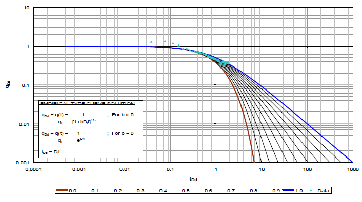
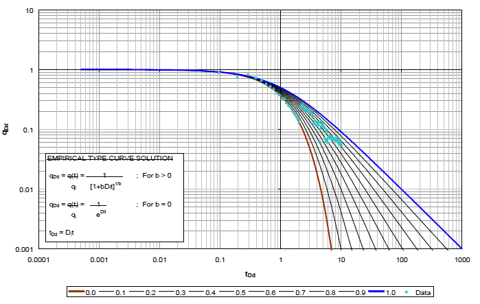
Figure 34: Type Curve BRN Gas
Figure 36: NPV calculator results BRN
The PVP curves which show trend of the NPV are shown below.
Both the curves show an inverse proportion.
DISCUSSION
The results obtained are now analysed so that predictions can be done.
CONCLUSION
In this project, we have used methods and designed wells for the company. The decline curve analysis method was used for determination of the initial rate of production, the hyperbolic exponent, the initial nominal decline rate. We used this data to forecast the values for next three years. Using this forecast, we determined the values for monthly net cash flow. The net present values were determined using the software. The values obtained were $236,154 and $546,823. The said values represent the present value of three year forecast of production from these well. The other well must be selected if the purchase price is upto a maximum $310,669 more than the first one. However, if the price is more than $310,669 the first, then the first must be taken.
APPENDIX I: WORK DISTRIBUTION
The work distribution is shown in table below.
APPENDIX II: STANDARD CHARTS
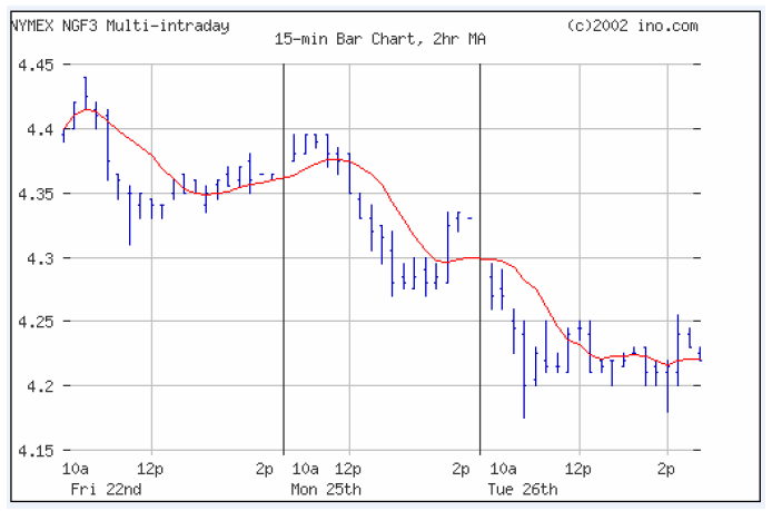
Figure 39: NYMEX NGF 3