
Then xax xax xax xax morgans law morgans law
Ethan D. Bloch
Proofs and Fundamentals
Editorial Board
S. Axler K.A. Ribet
Mathematics Department
San Francisco State University San Francisco, CA 94132
© Springer Science+Business Media, LLC 2011
All rights reserved. This work may not be translated or copied in whole or in part without the written permission of the publisher (Springer Science+Business Media, LLC, 233 Spring Street, New York, NY 10013, USA), except for brief excerpts in connection with reviews or scholarly analysis. Use in connection with any form of information storage and retrieval, electronic adaptation, computer software, or by similar or dissimilar methodology now known or hereafter developed is forbidden.The use in this publication of trade names, trademarks, service marks, and similar terms, even if they are not identified as such, is not to be taken as an expression of opinion as to whether or not they are subject to proprietary rights.
Preface to the Second Edition . . . . . . . . . . . . . . . . . . . . . . . . . . . . . . . . . . . . . . . . xi
Preface to the First Edition . . . . . . . . . . . . . . . . . . . . . . . . . . . . . . . . . . . . . . . . . . xiv
| 3.3 | |||
| 3.4 |
|
||
| 3.5 |
|
||
| 4 | |||
| 4.1 | |||
| 4.2 | |||
| 4.3 | |||
| 4.4 |
|
||
| 4.5 |
|
||
| 5 | |||
| 5.1 | |||
| 5.2 | |||
| 5.3 | |||
| 6 |
|
||
| 6.1 |
|
||
| 6.2 | |||
| 6.3 | |||
| 6.4 | |||
| 6.5 | |||
| 6.6 |
|
||
| 6.7 |
|
||
| 7 | |||
| 7.1 | |||
| 7.2 |
|
||
| 7.3 |
|
||
| 7.4 | |||
| 7.5 | |||
| 7.6 | |||
| 7.7 | |||
| 7.8 |
|
||
| 8 |
|
||
| 8.1 | |||
| 8.2 | |||
| 8.3 | |||
| 8.4 | |||
| 8.5 |
|
||
| 8.6 |
|
||
| 8.7 | |||
Though the bulk of the text has remained unchanged from the first edition, there are a number of changes, large and small, that will hopefully improve the text. As always, any remaining problems are solely the fault of the author.
Changes from the First Edition to the Second Edition
(3) The chapter on the construction of the natural numbers, integers and ratio-nal numbers from the Peano Postulates was removed entirely. That material was originally included to provide the needed background about the number systems, particularly for the discussion of the cardinality of sets in Chapter 6, but it was always somewhat out of place given the level and scope of this text. The background material needed for Chapter 6 has now been summarized in a new section at the start of that chapter, making the chapter both self-contained and more accessible than it previously was. The construction of the number systems from the Peano Postulates more properly belongs to a course in real analysis or in the foundations of mathematics; the curious reader may find this material in a variety of sources, for example [Blo11, Chapter 1].
(4) Section 3.4 on families of sets has been thoroughly revised, with the focus being on families of sets in general, not necessarily thought of as indexed.
(9) Many minor adjustments of wording have been made throughout the text, with the hope of improving the exposition.
Preface to the Second Edition xiii
My appreciation goes to Ann Kostant, now retired Executive Editor of Mathemat-ics/Physics at Birkh¨auser, for her unceasing support of this book, and to Elizabeth Loew, Senior Editor of Mathematics at Springer-Verlag, for stepping in upon Ann’s retirement and providing me with very helpful guidance. I would like to thank Shel-don Axler and Kenneth Ribet, the editors of Undergraduate Texts in Mathematics, for their many useful suggestions for improving the book. Thanks also go to Nathan Brothers and the copyediting and production staff at Springer-Verlag for their ter-rific work on the book; to Martin Stock for help with LATEX; and to Pedro Quaresma for assistance with his very nice LATEX commutative diagrams package DCpic, with which the commutative diagrams in this edition were composed.
I would very much like to thank the Einstein Institute of Mathematics at the Hebrew University of Jerusalem, and especially Professor Emanuel Farjoun, for their very kind hospitality during a sabbatical when this edition was drafted.
This text contains core topics that the author believes any transition course should cover, as well as some optional material intended to give the instructor some flexi-bility in designing a course. The presentation is straightforward and focuses on the essentials, without being too elementary, too excessively pedagogical, and too full of distractions.
Some of the features of this text are the following:
(4) The material is presented in the way that mathematicians actually use it rather than in the most axiomatically direct way. For example, a function is a special type of a relation, and from a strictly axiomatic point of view, it would make sense to treat relations first, and then develop functions as a special case of relations. Most mathematicians do not think of functions in this way (except perhaps for some combinatorialists), and we cover functions before relations, offering clearer treatments of each topic.
(5) A section devoted to the proper writing of mathematics has been included, to help remind students and instructors of the importance of good writing.
Part III, Extras, consists of Chapters 7 and 8, and has brief treatments of a variety of topics, including groups, homomorphisms, partially ordered sets, lattices, combi-natorics and sequences, and concludes with additional topics for exploration by the reader, as well as a collection of attempted proofs (actually submitted by students) which the reader should critique as if she were the professor.
Some instructors might choose to skip Section 4.5 and Section 6.4, the former be-cause it is very abstract, and the latter because it is viewed as not necessary. Though skipping either or both of these two sections is certainly plausible, instructors are urged to consider not to do so. Section 4.5 is intended to help students prepare for dealing with sets of linear maps in linear algebra, and comparable constructions in other branches of mathematics. Section 6.4 is a topic that is often skipped over in the mathematical education of many undergraduates, and that is unfortunate, because
Thanks go to the following individuals for their valuable assistance, and ex-tremely helpful comments on various drafts: Robert Cutler, Peter Dolan, Richard Goldstone, Mark Halsey, Leon Harkleroad, Robert Martin, Robert McGrail and Lau-ren Rose. Bard students Leah Bielski, AmyCara Brosnan, Sean Callanan, Emilie Courage, Urska Dolinsek, Lisa Downward, Brian Duran, Jocelyn Four´e, Jane Gilvin, Shankar Gopalakrishnan, Maren Holmen, Baseeruddin Khan, Emmanuel Kypraios, Jurvis LaSalle, Dareth McKenna, Daniel Newsome, Luke Nickerson, Brianna Nor-ton, Sarah Shapiro, Jaren Smith, Matthew Turgeon, D. Zach Watkinson and Xiaoyu Zhang found many errors in various drafts, and provided useful suggestions for im-provements.
My appreciation goes to Ann Kostant, Executive Editor of Mathematics/Physics at Birkh¨auser, for her unflagging support and continual good advice, for the second time around; thanks also to Elizabeth Loew, Tom Grasso, Amy Hendrickson and Martin Stock, and to the unnamed reviewers, who read through the manuscript with eagle eyes. Thanks to the Mathematics Department at the University of Pennsylva-nia, for hosting me during a sabbatical when parts of this book were written. The commutative diagrams in this text were composed using Paul Taylor’s commutative diagrams package.
To the Student
This book is designed to bridge the large conceptual gap between computational courses such as calculus, usually taken by first- and second-year college students, and more theoretical courses such as linear algebra, abstract algebra and real anal-ysis, which feature rigorous definitions and proofs of a type not usually found in calculus and lower-level courses. The material in this text was chosen because it is, in the author’s experience, what students need to be ready for advanced mathematics courses. The material is also worth studying in its own right, by anyone who wishes to get a feel for how contemporary mathematicians do mathematics.
Prerequisites
A course that uses this text would generally have as a prerequisite a standard calculus sequence, or at least one solid semester of calculus. In fact, the calculus prerequisite is used only to insure a certain level of “mathematical maturity,” which means suf-ficient experience—and comfort — with mathematics and mathematical thinking. Calculus per se is not used in this text (other than an occasional reference to it in the exercises); neither is there much of pre-calculus. We do use standard facts about numbers (the natural numbers, the integers, the rational numbers and the real num-bers) with which the reader is certainly familiar. See the Appendix for a brief list of some of the standard properties of real numbers that we use. On a few occasions we will give an example with matrices, though such examples can easily be skipped.
To the Student xxi
Mathematical Notation and Terminology
What This Text Is Not
Mathematics as an intellectual endeavor has an interesting history, starting in such ancient civilizations such as Egypt, Greece, Babylonia, India and China, progressing through the Middle Ages (especially in the non-Western world), and accelerating up until the present time. The greatest mathematicians of all time, such as Archimedes,
To the Instructor
There is an opposing set of pedagogical imperatives when teaching a transition course of the kind for which this text is designed: On the one hand, students often need assistance making the transition from computational mathematics to abstract mathematics, and as such it is important not to jump straight into water that is too deep. On the other hand, the only way to learn to write rigorous proofs is to write rigorous proofs; shielding students from rigor of the type mathematicians use will only ensure that they will not learn how to do mathematics properly.
One place where too much indulgence is given, however, even in more advanced mathematics courses, and where such indulgence is, the author believes, quite mis-guided, involves the proper and careful writing of proofs. Seasoned mathematicians make honest mathematical errors all the time (as we should point out to our students), and we should certainly understand such errors by our students. By contrast, there is simply no excuse for sloppiness in writing proofs, whether the sloppiness is physical (hastily written first drafts of proofs handed in rather than neatly written final drafts) or in the writing style (incorrect grammar, undefined symbols, etc.). Physical sloppi-ness is often a sign of either laziness or disrespect, and sloppiness in writing style is often a mask for sloppy thinking.
The elements of writing mathematics are discussed in detail in Section 2.6. It is suggested that these notions be used in any course taught with this book (though of course it is possible to teach the material in this text without paying attention to proper writing). The author has heard the argument that students in an introductory course are simply not ready for an emphasis on the proper writing of mathematics, but his experience teaching says otherwise: not only are students ready and able to write carefully no matter what their mathematical sophistication, but they gain much from the experience because careful writing helps enforce careful thinking. Of course, students will only learn to write carefully if their instructor stresses the importance of writing by word and example, and if their homework assignments and tests include comments on writing as well as mathematical substance.
Logic is the hygiene the mathematician practices to keep his ideas healthy and strong.
– Hermann Weyl (1885–1955)
E.D. Bloch, Proofs and Fundamentals: A First Course in Abstract Mathematics, 3
Undergraduate Texts in Mathematics, DOI 10.1007/978-1-4419-7127-2_1, © Springer Science+Business Media, LLC 2011
1.2 Statements
When we prove theorems in mathematics, we are demonstrating the truth of certain statements. We therefore need to start our discussion of logic with a look at state-ments, and at how we recognize certain statements as true or false. A statement is anything we can say, write or otherwise express that is either true or false. For ex-ample, the expression “Fred Smith is twenty years old” is a statement, because it is either true or false. We might not know whether this statement is actually true or not, because to know that would require that we know some information about Fred Smith, for example his date of birth, and that information might not be available to us. For something to be a statement, it has to be either true or false in principle; it does not matter whether we personally can verify its truth or falsity. By contrast, the expression “Eat a pineapple” is not a statement, because it cannot be said to be either true or false.
| 1.2 Statements | 5 |
|---|---|
For our definitions of these five constructions, we let P and Q be statements. the statement that, intuitively, is true if both P and Q are true, and is false otherwise. Our first construction, the conjunction of P and Q, which is denoted P ∧ Q, is . This truth table, and all others like it, shows whether the new statement (in this case P∧Q) is true or false for each possible combination of the truth or falsity of each of P and Q. |
|
| 6 | |
|---|---|
the statement that, intuitively, is true if either P is true or Q is true or both are true, Our second construction, the disjunction of P and Q, which is denoted P∨Q, is and is false otherwise. We read P∨Q as “P or Q.” The precise definition of P∨Q is given by the truth table The truth of the statement P∨Q means that at least one of P or Q is true. Though we write P∨Q in English as “P or Q,” it is very important to distinguish the mathe-matical use of the word “or” from the colloquial use of the word. The mathematical use of the word “or” always means an inclusive “or,” so that if “P or Q” is true, then either P is true, or Q is true, or both P and Q are true. By contrast, the colloquial use of the word “or” often means an exclusive “or,” which does not allow for both P and Q to be true. In this text, as in all mathematical works, we will always mean an inclusive “or,” as given in the truth table above. A simple example of a disjunction is the statement “my car is red or it will rain today.” This statement has the form P ∨ Q, where P = “my car is red,” and Q = “it will rain today.” The truth of this statement implies that at least one of the statements“my car is red” or “it will rain today” is true. The only thing not allowed is that both“my car is red” and “it will rain today” are false. |
|
as “Not Susan likes mushy bananas,” both because that is not proper English, and Let P = “Susan likes mushy bananas.” It would not work in English to write ¬P
because it appears as if the subject of the sentence is someone named
“Not Susan.”The most straightforward way of negating P is to
write ¬P = “it is not the case that Susan likes mushy bananas.”
While formally correct, this last statement is quite awkward to read,
and it is preferable to replace it with an easier-to-read expression,
for example “Susan does not like mushy bananas.”
Our final two ways of combining statements, both of which are connected
to the idea of logical implication, are slightly more subtle than what
we have seen so far. Consider the statement “If Fred goes on vacation,
he will read a book.” What would it mean to say that this statement is
true? It would not mean that Fred is going on vacation, nor would it
mean that Fred will read a book. The truth of this statement means only
that if one thing happens (namely, Fred goes on vacation), then another
thing will happen (namely, Fred reads a book). In other words, the one
way in which this statement would be false would be if Fred goes on
vacation, but does not read a book. The truth of this statement would
not say anything about whether Fred will or will not go on vacation, nor
would it say anything about what will happen if Fred does not go on
vacation. In particular, if Fred did not go on vacation, then it would
not contradict this statement if Fred read a book nonetheless.
1.2 Statements 9
| 1.2 Statements | 11 | ||||
|---|---|---|---|---|---|
An example of a tautology is the statement “Irene has red hair or she does not have red hair.” It seems intuitively clear that this statement is a tautology, and we can verify this fact formally by using truth tables. Let P = “Irene has red hair.” Then our purported tautology is the statement P∨¬P. The truth table for this statement is
The statement “Irene has red hair and she does not have red hair” is a contradic-tion. In symbols this statement is P∧¬P, and it has truth table |
|||||
| 12 |
|
|---|---|
tuitively reasonable. It is possible, however, to have more complicated (and not so That P ∨ ¬P is a tautology, and that P ∧ ¬P is a contradiction, seems quite in- 7 . We see in column 11 that the statement [(P ∧ Q) →
R] → [P → (Q → R) is always true,
regardless of whether each of P, Q and R is
true or false. Hence the statement is a tautology. Suppose that
P = “Sam is sad,” let Q = “Warren is sad” and
R =“Sam and Warren eat pasta.” Then the statement becomes “If
it is true that if Sam and Warren are both sad then they eat pasta, then
it is true that if Sam is sad, then if Warren is sad they eat
pasta.” |
|
(4) The U.S. has 49 states.
(5) I like to eat fruit, and you often think about traveling to Spain. (6) If we go out tonight, the babysitter will be unhappy.
(4) x+y = z.
(5) (a+b)2= a2+2ab+b2. (6) a2+b2= c2.
|
1.2 Statements | 13 |
|---|---|---|
(1) Z → X.
(2) X ↔︎ Y.
(1) Fred does not like to eat figs.
(2) Fred has red hair, and does not have a big nose.
(7) It is not the case that Fred has a big nose, or he has red hair.
(8) Fred has a big nose and red hair, or he has a big nose and likes to eat figs.
(4) The house is not ugly if and only if it is 30 years old.
(5) The house is 30 years old if it is blue, and it is not ugly if it is 30 years old. (6) For the house to be ugly, it is necessary and sufficient that it be ugly and 30 years old.
(5) (D∧A)∨(B∧C).
(6) C ∨[D∨(A∧B)].
Exercise 1.2.8. Suppose that X is a false statement, that Y is a true statement, that Z is a false statement and that W is a true statement. Which of the following statements are true, and which are false?
(4) W → (X → ¬W).
(5) [(Y → W) ↔︎ W]∧¬X. (6) (W → X) ↔︎ ¬(Z ∨Y).
(4) Flora likes fruit or nuts, and she likes carrots or rutabagas.
(5) Flora likes rutabagas, or she likes fruit and either carrots or rutabagas.
(5) If Hector likes lentils then he likes sunflower seeds, or Hector likes lentils if and only if he likes peas.
(6) For Hector to like beans and lentils it is necessary and sufficient for him to like peas or sunflower seeds.
Exercise 1.2.12. Make a truth table for each of the following statements.
(1) X → ¬Y.
(1) P∨(¬P∧Q).
(2) (X ∨Y) ↔︎ (¬X → Y).
(7) [(P ↔︎ ¬Q)∧P]∧Q.
Exercise 1.2.14. Which of the following statements are tautologies, which are con-tradictions and which are neither?
(6) The cow is green or the cow is not green, if and only if the goat is blue and the goat is not blue.
Exercise 1.2.15. Let P be a statement, let T be a tautology and let C be a contradic-tion.
The two examples of relations between statements given above represent the two types of such relations we will study, namely, implication and equivalence, which are the meta-statement analogs of conditionals and biconditionals. We start with im-plication.
The intuitive idea of logical implication is that statement P implies statement Q if necessarily Q is true whenever P is true. In other words, it can never be the case that
| P | Q | P ∨ Q |
|---|---|---|
|
|
statement [¬(P → Q)] → (P∨Q) will be a tautology (also in Section 1.2), as can be
1.3 Relations Between Statements 17
We see in Column 8 that the statement [¬(P → Q)] → (P ∨ Q) is always true, and hence it is indeed a tautology.
situations where P → Q is not just a statement (which is always the case), but where P → Q is a tautology. Moreover, we will see in Section 1.4 that implications of statements will be extremely useful in constructing valid arguments. In particular,
|
|---|
(Simplification).
(Addition).
(Hypothetical Syllogism).
(Conditional-Biconditional).
| P | Q | [(P → Q) ∧ P] → Q |
|---|---|---|
|
We see in Column 7 that the statement [(P → Q)∧P] → Q is always true, and hence it is a tautology. ///
What interests us are logically equivalent statements that are not simply English variants of the same symbolic statement, but rather are truly different statements. For example, the statement “it is not that case that I do not own a bicycle” will be seen to be equivalent to “I own a bicycle.” If we let P = “I own a bicycle,” then the statement“it is not that case that I do not own a bicycle” is ¬(¬P). This statement is not identi-cal to P. It will be very important to us to be able to recognize that some non-identical statements, for example ¬(¬P) and P, are in fact logically equivalent. Such equiv-alences will allow us to find alternative forms of the statements of some theorems, and these alternative forms are sometimes easier to prove than the originals.
The intuitive idea of equivalence of statements is that to claim that statements P and Q are equivalent means that necessarily P is true if and only if Q is true. Necessity is once again the key here, as can be seen once more using the statements
(Commutative Law).
(Commutative Law).
| 20 | |
|---|---|
(Distributive Law).
|
|
We see in Column 13 that the statement[P∨(Q∧R)] ↔︎ [(P∨Q)∧(P∨R)], and hence it is a tautology. ///
Part (1) of Fact 1.3.2 might appear innocuous, but this equivalence plays a very important role in standard mathematical proofs. In informal terms, the equivalence of ¬(¬P) and P means that “two negatives cancel each other out.” From the point of view of constructing mathematical proofs, suppose that we want to show that a statement P is true. One method to prove this statement would be to hypothesize that¬P is true, and derive a contradiction. It would then follow that ¬P is false, which implies that ¬(¬P) is true. Because ¬(¬P) and P are equivalent, it would follow that P is true. This methodology of proof might sound rather convoluted, but it is often quite useful, and is called proof by contradiction. A detailed discussion of this method of proof is in Section 2.3.
tant for constructing mathematical proofs, as seen in Section 2.3, relevant terminol-Because the equivalence of the statements P → Q and ¬Q → ¬P will be so impor-
ogy is merited. Given a conditional statement of the form P → Q, we call ¬Q → ¬P the contrapositive of the original statement. For example, the contrapositive of “if I eat too much I will feel sick” is “if I do not feel sick I did not eat too much.”Fact 1.3.2 (9) says that a statement and its contrapositive are always equivalent.
| Exercises |
|---|
Exercise 1.3.1. Let P, Q, R and S be statements. Show that the following are true.
(1) ¬(P → Q) ⇒ P.
(6) (P ↔︎ R)∧(Q ↔︎ S) ⇒ (P∨Q) ↔︎ (R∨S).
Exercise 1.3.2. [Used in Exercise 1.3.12 and Section 2.4.] Let P, Q, A and B be state-ments. Show that the following are true.
1.3 Relations Between Statements 23
Exercise 1.3.3. Let P be a statement, let T be a tautology and letC be a contradiction.
Exercise 1.3.5. For each pair of statements, determine whether or not the two state-ments are equivalent.
(1) “If it rains, then I will see a movie”; and “it is not raining or I will see a movie.”
(2) “This shirt has stripes, and it has short sleeves or a band collar”; and “this shirt has stripes and it has short sleeves, or it has a band collar.”
(3) “It is not true that I like apples and oranges”; and “I do not like apples and I do not like oranges.”
(4) “The cat is gray, or it has stripes and speckles”; and “the cat is gray or it has stripes, and the cat is gray or it has speckles.”
(5) “It is not the case that: melons are ripe if and only if they are soft to the touch”; and “melons are ripe and soft to the touch, or they are not ripe or not soft to the touch.”
(2) I will go home if it is after midnight.
(3) Good fences make good neighbors.
Exercise 1.3.10. Negate each of the following statements.
(1) e5> 0. (4) If y = 3 then y2= 7.
(4) If I tell you a joke, you will smile.
(5) The play will end on time if and only if the actors are in good spirits. (6) The room will get painted if you buy the paint.
(1) The operations ∧ and ∨ are examples of binary logical operations, in that they take two inputs and give one output; the operation ¬ is an example of a unary logical operation, in that it takes one input and gives one output. How many possible unary and binary logical operations are there? List all of them using truth tables, and give the familiar names to those that we have already seen.
| 1.4 Valid Arguments | 25 |
|---|---|
.
|
|
If the poodle-o-matic is cheap or is energy efficient, then it will not make money for the manufacturer. If the poodle-o-matic is painted red, then it will make money for the manufacturer. The poodle-o-matic is cheap. Therefore the poodle-o-matic is not painted red.
This collection of statements is an example of a logical argument, which in general is a collection of statements, the last of which is the conclusion of the argument, and the rest of which are the premises of the argument. Clearly, the use of the word“argument” in logic is different from the colloquial use of the word, where it could
|
P → Q P | Modus Tollendo Ponens |
|
|---|---|---|---|
| Modus Tollendo Ponens | |||
|
|||
|
Biconditional-Conditional | ||
| P ↔︎ Q | |||
|
Biconditional-Conditional | P → Q | |
|
|||
| P ↔︎ Q | |||
| Conditional-Biconditional | Q → P | ||
| P → Q Q → P | |||
|
|
P ↔︎ Q | |
| Hypothetical Syllogism | |||
| P → Q Q → R | |||
|
Constructive Dilemma | P → R | |
|
P → Q R → S | ||
|
|||
|
|||
A few of the rules of inference listed above were not treated in Fact 1.3.1, al-though they are easily seen to be true. Double Negation is proved in Fact 1.3.2, although here we state it as two implications, rather than one equivalence. Repetition ence. Adjunction is just a glorified version of repetition, because if we stated it in the is evidently true (because P → P is a tautology), but is still useful as a rule of infer-format of Fact 1.3.1, it would look like P∧Q ⇒ P∧Q. We now return to our argument concerning the poodle-o-matic. Using the rules of inference listed above, we can construct a justification for the argument. We use here the two-column format that may be familiar from high school geometry proofs,
28 1 Informal Logic
This sort of justification, often referred to by logicians as a derivation, is a chain of statements connected by meta-statements (namely, the justifications for each line). If an argument has a derivation, we say that the argument is derivable. Observe that the derivability of an argument is one thing, and the truth of the component statements involved is another. We can have a derivable argument with component statements that happen to be true, or happen to be false, and we can have a non-derivable argument with component statements that happen to be true, or happen to be false. The derivability of an argument is only a question of the relation of the conclusion of the argument with the premises, not whether the conclusion or premises are actually true.
For a given argument, there is often more than one possible derivation. The fol-lowing is another derivation for the poodle-o-matic argument, this time making use of the equivalences of statements given in Fact 1.3.2, in addition to our rules of infer-ence. In general, it is acceptable in a derivation to replace one statement with another that is equivalent to it. The alternative derivation is
We now face an important question: given an argument, we have two notions of whether the argument works, which are that it is or is not valid, and that it is or is not derivable. The former notion involves checking truth values (which is done with truth tables), the latter constructing a chain of statements linked by rules of in-ference. What is the relation between these two approaches? Though it is not at all obvious, nor easy to prove, it turns out quite remarkably that these two approaches, while different in nature, always yield the same result. That is, an argument is valid
1.4 Valid Arguments 29
Jethro does not play the guitar, or Susan plays the flute. If Leslie does not play the xylophone, then Susan does not play the flute. Jethro plays the gui-tar, and Leslie does not play the xylophone. Therefore Ferdinand plays the accordion.
The strange thing about this argument is that there is no apparent connection between the conclusion and the premises. However, try as you might, you will not be able to find truth values for the component statements used in the argument for which the premises are all true but the conclusion is false. The argument is in fact valid, as odd as that might appear. Let J = “Jethro plays the guitar,” let S = “Susan plays the flute,”let L = “Leslie plays the xylophone” and let F = “Ferdinand plays the accordion.”A derivation for this argument is
The moral of this story is that we should avoid arguments that have premises that form contradictions. Such premises are often called inconsistent. Premises that are not inconsistent are called consistent. It is not that there is anything logically wrong with inconsistent premises, they are simply of no use to mathematicians, because we can derive anything from them. For example, when non-Euclidean geometry was first discovered in the early nineteenth century, it was important to determine whether the proposed axiom system for such geometry was consistent or not. In many mathemat-ical situations, for example geometry, it is not possible to demonstrate consistency directly via truth tables and the like, but it was eventually shown that non-Euclidean is no less consistent than Euclidean geometry. Because Euclidean geometry is so well studied and so widely used, and its consistency is not generally doubted, it followed that non-Euclidean geometry was no less worthwhile mathematically than Euclidean geometry. See [Tru87, Chapter 7] for details.
Whereas arguments with inconsistent premises are not logically flawed, but rather do not allow for any useful conclusions, we often do encounter logical er-rors in both formal and informal argumentation. We conclude this section with a brief mention of a few common logical errors, often referred to as fallacies, that are regularly found in attempted mathematical proofs (and elsewhere).
Again this argument is invalid. The first premise says what we could conclude if the senator does a certain thing, namely, votes himself a raise. It does not say anything if that certain thing does not happen. Therefore, just because the senator did not vote himself a raise, we cannot conclude anything about his character—there could be many other things that might raise questions about him. In symbols, the argument here is (P → Q) ∧ ¬P ⇒ ¬Q. Again, there is no such implication, as can be seen by checking the appropriate truth table. This fallacy is known as the fallacy of the inverse (and is also known as the fallacy of denying the antecedent).
The third type of error we mention is of a slightly different nature. Consider the following argument.
| Exercises |
|---|
Exercise 1.4.1. For each of the following arguments, if it is valid, give a derivation, and if it is not valid, show why.
Exercise 1.4.2. For each of the following arguments, if it is valid, give a derivation, and if it is not valid, show why.
(4) If Susan likes fish, then she likes onions. If Susan does not like garlic, then she does not like onions. If she likes garlic, then she likes guavas. She likes fish or she likes cilantro. She does not like guavas. Therefore, Susan likes cilantro.
(5) It is not the case that Fred plays both guitar and flute. If Fred does not play guitar and he does not play flute, then he plays both organ and harp. If he plays harp, then he plays organ. Therefore Fred plays organ.
(3) It is not the case that clothes are annoying or not cheap. Clothes are not cheap or they are unfashionable. If clothes are unfashionable they are silly. There-fore clothes are silly.
(4) If music soothes the soul then souls have ears. Music soothes the soul or musicians are calm. It is not the case that souls have ears or musicians are calm. Therefore musicians have souls.
(3) The cow moos whenever the pig oinks. The cow moos. Therefore the pig oinks.
(4) A nice day is sufficient for frolicking children or napping adults. Adults are napping. Therefore it is a nice day.
Our discussion of logic so far has been missing one crucial ingredient used in the formulation of theorems and proofs. We often encounter in mathematics expressions such as “x3≥ 8,” which we might wish to prove. This expression as written is not precise, however, because it does not state which possible values of x are under con-sideration. Indeed, the expression is not a statement. A more useful expression, which is a statement, would be “x3≥ 8, for all real numbers x ≥ 2.” The phrase “for all real numbers x ≥ 2” is an example of a quantifier. The other type of quantifier commonly used is the first part of the statement “there exists a real number x such that x2= 9.”What is common to both these phrases is that they tell us about the variables under consideration; they tell us what the possible values of the variable are, and whether the statement involving the variable necessarily holds for all possible values of the variable or only for some values (that is, one or more value).
The use of quantifiers vastly expands the range of possible statements that can be formed in comparison with the statements that were made in previous sections of this chapter. Quantifiers are so important that the type of logic that involves quantifiers has its own name, which is “first-order” (and is also known as “predicate”) logic; the type of logic we looked at previously is called “sentential” (and is also known as“propositional”) logic.
As a preliminary to our discussion of quantifiers, consider the expression P =“x + y > 0.” Observe that x and y have the same roles in P. Using P we can form a new expression Q = “for all positive real numbers x, the inequality x+y > 0 holds.”In contrast to P, there is a substantial difference between the roles of x and y in Q. The symbol x is called a bound variable in Q, in that we have no ability to choose which values of x we want to consider. By contrast, the symbol y is called a free variable in Q, because its possible values are not limited. Because y is a free variable in Q, it is often useful to write Q(y) instead of Q to indicate that y is free. In P both x and y are free variables, and we would denote that by writing P(x,y).
The difference between a bound variable and a free one can be seen by changing the variables in Q. If we change every occurrence of x to w in Q, we obtain ˆQ =“for all positive real numbers w, the inequality w + y > 0 holds.” For each possible value of y, we observe that ˆQ and Q have precisely the same meaning. In other words, if Q were part of a larger expression, then the larger expression would be entirely unchanged by replacing Q with ˆQ. By contrast, suppose that we change every occurrence of y to z in Q, obtaining ˜Q = “for all positive real numbers x, the inequality x + z > 0 holds.” Then ˜Q does not have the same meaning as Q, because y and z (over which we have no control in Q and ˜Q respectively) might be assigned different values, for example if Q were part of a larger expression that had both y and z appearing outside Q. In other words, changing the y to z made a difference precisely because y is a free variable in Q.
36 1 Informal Logic
be the case that P(x) is true for some values of x that are not in U, but we cannot tell that from the statement as written.
For the sake of completeness, we need to allow the case where the collection U has nothing in it. In that case, the statement (∀x in U)P(x) is always true, no matter what P(x) is, for the following reason. The statement “(∀x in U)P(x)” is equivalent to the statement “if x is in U, then P(x) is true.” When the collection U has nothing in it, then the statement “x is in U” is false, and hence the conditional statement “if x is in U, then P(x) is true” is true.
For the other type of quantifier we are interested in, once again let P(x) be a statement with free variable x, and let U denote a collection of possible values of x. An existential quantifier applied to P(x) is the statement, denoted (∃x in U)P(x), which is true if P(x) is true for at least one value of x in U. If the collection U is understood from the context, then we will write (∃x)P(x). Observe that if the It is important to note that the phrase “at least one value of x in U” means one or collection U has nothing in it, then the statement (∃x)P(x) is false.
Let Q(r) = “person r has brown hair,” and let W be the collection of all people in the world. Then the statement (∃r in W)Q(r) would mean that “there is some-one with brown hair,” or equivalently “some people have brown hair” (which is a true statement). Let E(m) = “m is an even number” and let M(m) = “m is a prime number,” where the collection of possible values of m is the integers. The statement“some integers are even and prime” can be expressed symbolically by first rephras-ing it as “there exists x such that x is even and x is prime,” which is (∃x)[E(x)∧M(x)] (this statement is true, because 2 is both even and prime).
The reader might wonder why we use only the above two types of quantifiers, and whether other quantifiers are needed. For example, the statement “no dog likes cats” clearly has a quantifier, but which quantifier is it? If we let U be the collection of all dogs, and if we let P(x) = “dog x likes cats,” then our statement is “there is no x in U such that P(x).” However, the expression “there is no x in U,” though certainly a quantifier of some sort, is neither a universal quantifier nor an existential quantifier. Fortunately, rather than needing to define a third type of quantifier to be able to handle the present statement, we can rewrite our statement in English as “every dog does not like cats,” and in symbols that becomes (∀x in U)(¬P(x)). In general, all the quantification that we need in mathematics can be expressed in terms of universal quantifiers and existential quantifiers.
38 1 Informal Logic
lead to mistakes in proving theorems that have statements with multiple quantifiers. A very important occurrence of the importance of the order of multiple quantifiers is in the “ε-δ” proofs treated in real analysis courses; see Section 7.8 for a similar type of proof from real analysis, and see any introductory real analysis text for a detailed discussion of ε-δ proofs.
(3) (∀x)(∃y)L(x,y). This statement can be written as “for each person x, there is a type of fruit y such that x likes to eat y,” and more simply as “every person likes at least one type of fruit.” To verify whether this statement is true, we would have to ask each person in the world if she likes some type of fruit; if at least one person does not like any type of fruit, then the statement would be false.
(4) (∃x)(∀y)L(x,y). This statement can be written as “there is a person x such that for all types of fruit y, person x likes to eat y,” and more simply as “there is a person who likes every type of fruit.” To verify whether this statement is true, we would start asking one person at a time if she likes every type of fruit; as soon as we found one person who answers yes, we would know that the statement is true, and we could stop asking more people. If no such person is found, then the statement would be false.
(7) (∃x)(∃y)L(x,y). This statement can be written as “there is a person x such that there is a type of fruit y such that x likes to eat y,” and more simply as“there is a person who likes at least one type of fruit.” To verify whether this statement is true, we would have to start asking one person at a time if she likes some type of fruit; as soon as we found one person who answers yes, we would know that the statement is true, and we could stop asking more people.
(8) (∃y)(∃x)L(x,y). This statement can be written as “there is a type of fruit y such that there is a person x such that x likes to eat y,” and more simply as“there is a type of fruit that is liked by at least one person.” This statement is equivalent to Statement 7.
40 1 Informal Logic
to recognize that ¬Q is not the same as the statement “all people do not have red hair,” which in symbols would be written (∀x)(¬P(x)). This last statement is much stronger than is needed to say that Q is false. The effect of the negation of Q is to change the quantifier, as well as to negate the statement being quantified.
1. ¬[(∀x in U)P(x)] ⇔ (∃x in U)(¬P(x)).
2. ¬[(∃x in U)P(x)] ⇔ (∀x in U)(¬P(x)).
¬Q ⇔ ¬[(∀w)(∃y)P(w,y)] ⇔ (∃w)¬[(∃y)P(w,y)] ⇔ (∃w)(∀y)(¬P(w,y)).
Rephrasing this last expression in English yields ¬Q = “there exists a real number w such that for all real numbers y, the relation f(y) ̸= w holds.” It is often easier to negate statements with multiple quantifiers by first translating them into symbolic form, negating them symbolically and then translating back into English. With a bit of practice it is possible to negate such statements directly in English as well, as long as the statements are not too complicated. |
|
|---|---|
| Universal Instantiation | |
where b is something of U, and where the symbol “b” does not already have any other meaning in the given argument.
of inference will be used regularly in our mathematical proofs. See [Cop68, Chap-ter 10] for further discussion of these rules of inference.
An example of a simple logical argument involving quantifiers is the following.
|
|
|---|---|
Exercise 1.5.1. Suppose that the possible values of x are all people. Let Y(x) =“x has green hair,” let Z(x) = “x likes pickles” and let W(x) = “x has a pet frog.”Translate the following statements into words.
1.5 Quantifiers 43
Exercise 1.5.2. Suppose that the possible values of x and y are all cars. Let L(x,y) =“x is as fast as y,” let M(x,y) = “x is as expensive as y” and let N(x,y) = “x is as old
as y.” Translate the following statements into words.
(2) All cows are four years old.
(3) There is a brown cow with white spots.
(1) There is a fruit such that all fruit taste better than it.
(2) For every fruit, there is a fruit that is riper than it.
(3) Cats like eating fish and taking naps.
(4) I liked one of the books I read last summer. (5) No one likes ice cream and pickles together.
(3) The equation x2−2x > 0 holds for all real numbers x. (4) Every parent has to change diapers.
(5) Every flying saucer is aiming to conquer some galaxy.
(9) At least one person in New York City owns every book published in 1990.
Exercise 1.5.7. Negate the following statement: There exists an integer Q such that for all real numbers x > 0, there exists a positive integer k such that ln(Q − x) > 5 and that if x ≤ k then Q is cacophonous. (The last term used in this exercise is meaningless.)
gelatinous real number x? (The terms used in this exercise are meaningless.)
Exercise 1.5.10. Someone claims that the argument
Find the flaw(s) in the derivation. |
|---|
(1), Existential Instantiation (3), Simplification
(2), Existential Instantiation (5), (4), Adjunction
(6), Existential Generalization.
| 1.5 Quantifiers | 45 | |
|---|---|---|
| (2) | ||
| (3) | ||
| (4) |
|
|
| Exercise 1.5.12. Write a derivation for each of the following arguments. | ||
(1) Every fish that is bony is not pleasant to eat. Every fish that is not bony is slimy. Therefore every fish that is pleasant to eat is slimy.
2
Strategies for Proofs
Be the above as it may, the importance of proofs should be put in the proper perspective. Intuition, experimentation and even play are no less important in today’s mathematical climate than rigor, because it is only by our intuition that we decide what new results to try to prove. The relation between intuition and formal rigor is not a trivial matter. Formal proofs and intuitive ideas essentially occupy different realms,
E.D. Bloch, Proofs and Fundamentals: A First Course in Abstract Mathematics, 4 7
Mathematics has moved over time in the direction of ever greater rigor, though why that has happened is a question we leave to historians of mathematics to explain. We can, nonetheless, articulate a number of reasons why mathematicians today use proofs. The main reason, of course, is to be sure that something is true. Contrary to popular misconception, mathematics is not a formal game in which we derive theorems from arbitrarily chosen axioms. Rather, we discuss various types of mathe-matical objects, some geometric (for example, circles), some algebraic (for example, polynomials), some analytic (for example, derivatives) and the like. To understand these objects fully, we need to use both intuition and rigor. Our intuition tells us what is important, what we think might be true, what to try next and so forth. Unfor-tunately, mathematical objects are often so complicated or abstract that our intuition at times fails, even for the most experienced mathematicians. We use rigorous proofs to verify that a given statement that appears intuitively true is indeed true.
Another use of mathematical proofs is to explain why things are true, though not every proof does that. Some proofs tell us that certain statements are true, but shed no intuitive light on their subjects. Other proofs might help explain the ideas that underpin the result being proved; such proofs are preferable, though any proof, even if non-intuitive, is better than no proof at all. A third reason for having proofs in mathematics is pedagogical. A student (or experienced mathematician for that matter) might feel that she understands a new concept, but it is often only when attempting to construct a proof using the concept that a more thorough understanding emerges. Finally, a mathematical proof is a way of communicating to another person an idea that one person believes intuitively, but the other does not.
niently broken down into the two-column (statement-justification) format. Second, the mathematical ideas of the proof, not its logical underpinnings, are the main is-sue on which we want to focus, and so we do not even mention the rules of logical inference used, but rather mention only the mathematical justification of each step. Second, mathematicians who are not logicians, which means most mathematicians, find long strings of logical symbols not only unpleasant to look at, but in most cases rather difficult to follow. See [EFT94, pp. 70–71] for a fully worked out example of putting a standard mathematical proof in group theory into a two-column format using formal logic. The mathematical result proved in that example is given in Ex-ercise 7.2.8; see Sections 7.2 and 7.3 for a brief introduction to groups. One look at the difference between the mathematicians’ version of the proof and the logicians’version, in terms of both length and complexity, should suffice to convince the reader why mathematicians do things as they do.
To some extent mathematicians relate to proofs the way the general public often reacts to art—they know it when they see it. But a proof is not like a work of modern art, where self-expression and creativity are key, and all rules are to be broken, but rather like classical art that followed formal rules. (This analogy is not meant as an endorsement of the public’s often negative reaction to serious modern art—classical art simply provides the analog we need here.) Also similarly to art, learning to recog-nize and construct rigorous mathematical proofs is accomplished not by discussing the philosophy of what constitutes a proof, but by learning the basic techniques, studying correct proofs, and, most importantly, doing lots of them. Just as art criti-cism is one thing and creating art is another, philosophizing about mathematics and doing mathematics are distinct activities (though of course it helps for the practi-tioner of each to know something about the other). For further discussion about the conceptual nature of proofs, see [Die92, Section 3.2] or [EC89, Chapter 5], and for more general discussion about mathematical activity see [Wil65] or [DHM95].
Theorem 2.1.1 (Pythagorean Theorem). Let △ABC be a right triangle, with sides of length a, b and c, where c is the length of the hypotenuse. Then a2+b2= c2.
When asked what the Pythagorean Theorem says, students often state “a2+b2= c2.” This expression alone is not the statement of the theorem—indeed, it is not a statement at all. Unless we know that a, b and c are the lengths of the sides of a right triangle, with c the length of the hypotenuse, we cannot conclude that a2+b2= c2. (The formula a2+ b2= c2is never true for the sides of a non-right triangle.) It is crucial to state theorems with all their hypotheses if we want to be able to prove them.
informally familiar with these numbers. See the Appendix for a brief list of some of the standard properties of the real numbers.
We conclude this section with our first example of a proof. You are probably familiar with the statement “the sum of even numbers is even.” This statement can be viewed in the form P → Q if we look at it properly, because it actually says “if n and m are even numbers, then n + m is an even number.” To construct a rigorous proof of our statement (as well as the corresponding result for odd numbers), we first need precise definitions of the terms involved.
We are now ready to state and prove our theorem. This result may seem rather trivial, but our point here is to see a properly done proof, not to learn an exciting new result about numbers.
Theorem 2.1.3. Let n and m be integers.
Because k and j are integers, so is k + j. Hence m+n is even.
(2) & (3). These two parts are proved similarly to Part (1), and the details are left to the reader. ⊓⊔
An important consideration when writing a proof is recognizing what needs to be proved and what doesn’t. There is no precise formula for such a determination, but the main factor is the context of the proof. In an advanced book on number theory, it would be unnecessary to prove the fact that the sum of two even integers is even; it would be safe to assume that the reader of such a book would either have seen the proof of this fact, or could prove it herself. For us, however, because we are just learning how to do such proofs, it is necessary to write out the proof of this fact in detail, even though we know from experience that the result is true. The reasons to prove facts that we already know are twofold: first, in order to gain practice writing proofs, we start with simple results, so that we can focus on the writing, and not on mathematical difficulties; second, there are cases where “facts” that seem obviously true turn out to be false, and the only way to be sure is to construct valid proofs.
Though mathematical proofs are logical arguments, observe that in the proof of Theorem 2.1.3 we did not use the logical symbols we discussed in Chapter 1. In general, it is not proper to use logical symbols in the writing of mathematical proofs. Logical symbols were used in Chapter 1 to help us become familiar with informal logic. When writing mathematical proofs, we make use of that informal logic, but we write using standard English (or whatever language is being used).
Exercise 2.1.1. Reformulate each of the following theorems in the form P → Q. (The statements of the theorems as given below are commonly used in mathematics courses; they are not necessarily the best possible ways to state these theorems.) |
|---|
(4) ex+y= exey.
54 2 Strategies for Proofs
For example, each of the three parts of Theorem 2.1.3 is of the form P → Q. To prove theorems, we therefore need to know how to prove statements of the form P → Q. The simplest form of proof, which we treat in this section, is the most obvious one: assume that P is true, and produce a series of steps, each one following from the previous ones, which eventually lead to Q. This type of proof is called a direct proof. That this sort of proof deserves a name is because there are other approaches that can be taken, as we will see in Section 2.3. An example of a direct proof is the proof of Theorem 2.1.3.
(argumentation)
|
2.2 Direct Proofs | 55 |
|---|---|---|
| ⊓⊔ |
integer a divides the integer b.” For example, even though it is not sensible to write the fraction 7/0, it is perfectly reasonable to write the expression 7|0, because 7 does in fact divide 0, because 7 · 0 = 0. Because of this potential confusion, and also to avoid ambiguous expressions such as 1/2+3 (is that1 2+ 3 or 2+3?), we suggest writing all fractions asa brather than a/b.
We now have two simple results about divisibility. The proof of each theorem is preceded by scratch work, to show how one might go about formulating such a proof.
Compare the proof with the scratch work. The proof might not appear substan-tially better than the scratch work at first glance, and it might even seem a bit mys-terious to someone who had not done the scratch work. Nonetheless, the proof is better than the scratch work, though in such a simple case the advantage might not be readily apparent. Unlike the scratch work, the proof starts with the hypotheses and proceeds logically to the conclusion, using the definition of divisibility precisely as stated. Later on we will see examples where the scratch work and the proof are more strikingly different.
Theorem 2.2.3. Any integer divides zero.
In sum, there are two main steps to the process of producing a rigorous proof: formulating it and writing it. These two activities are quite distinct, though in some very simple and straightforward proofs you might formulate as you write. In most cases, you first formulate the proof (at least in outline form) prior to writing. For a difficult proof the relation between formulating and writing is essentially dialectical. You might formulate a tentative proof, try writing it up, discover some flaws, go back to the formulating stage and so on.
Exercise 2.2.1. Outline the strategy for a direct proof of each of the following state-ments (do not prove them, because the terms are meaningless).
| 57 |
|---|
(1) Prove that 1|n.
(2) Prove that n|n.
(1) Prove that n+m is divisible by 3.
(2) Prove that nm is divisible by 3.
Exercise 2.2.6. Let a, b, c, m and n be integers. Prove that if a|b and a|c, then a|(bm+cn).
There is no foolproof method for knowing ahead of time whether a proof on which you are working should be a direct proof or a proof by one of these other methods. Experience often allows for an educated guess as to which strategy to try first. In any case, if one strategy does not appear to bear fruit, then another strategy should be attempted. It is only when the proof is completed that we know whether a given choice of strategy works.
Both strategies discussed in this section rely on ideas from our discussion of equivalence of statements in Section 1.3. For our first method, recall that the contra-positive of P → Q, the statement ¬Q → ¬P, is equivalent to P → Q. Hence, in order
Proof. Suppose that Q is false.
...
Theorem 2.3.1. Let n be an integer. If n2is odd, then n is odd.
Scratch Work. If we wanted to use a direct proof, we would have to start with the
start such a proof by observing that if n is even, then there is some integer k such that
n = 2k, and we then compute n2in terms of k, leading to the desired result. ///
it is often helpful to the reader to have the method of proof stated explicitly.
looks similar to proof by contrapositive but is actually distinct from it, is proof by Another method of proof for theorems with statements of the form P → Q, which
by contradiction.
Recall from Section 1.3 that ¬(P → Q) is equivalent to P∧¬Q. Suppose that we could prove that P∧¬Q is false. It would follow that ¬(P → Q) is false, and hence that ¬(¬(P → Q)) is true. Then, using Double Negation (Fact 1.3.2 (1)), we could conclude that P → Q is true.
Proof. We prove the result by contradiction. Suppose that P is true and that Q is false.
...
Proof. We prove the result by contradiction. Suppose that a, b and c are non-negative consecutive integers other than 3, 4 and 5, and that a2+ b2= c2. Because a, b and c are not 3, 4 and 5, we know that a ̸= 3, and because the three numbers are con-secutive, we know that b = a + 1 and c = a + 2. From a2+ b2= c2we deduce that a2+(a+1)2= (a+2)2. After expanding and rearranging we obtain a2−2a−3 = 0. This equation factors as (a − 3)(a + 1) = 0. Hence a = 3 or a = −1. We have al- ⊓⊔ready remarked that a ̸= 3, and we know a is non-negative. Therefore we have a contradiction, and the theorem is proved.
Our next two theorems are both famous results that have well-known proofs by contradiction. These clever proofs are much more difficult than what we have seen so far, and are more than would be expected of a student to figure out on her own at this point.
| 2.3 Proofs by Contrapositive and Contradiction | 61 | |
|---|---|---|
| that there is a positive real number x such that x2= 2 (and there is only one such number), but unfortunately it is beyond the scope of this book to give a proof of that fact. The proof requires tools from real analysis; see [Blo11, Theorem 2.6.9] for a | ||
| proof. | √2 exists, however, we can prove here that this number is irra- | |
|
||
62 2 Strategies for Proofs
The first few prime numbers are 2,3,5,7,11,.... The study of prime numbers is quite old and very extensive; see any book on elementary number theory, for example [Ros05], for details.
Theorem 2.3.7. There are infinitely many prime numbers.
Preliminary Analysis. We have not yet seen a rigorous treatment of what it means for there to be infinitely many of something, and so for now we need to use this concept in an intuitive fashion. A thorough discussion of finite vs. infinite is found in Chapter 6. The essential idea discussed in that chapter is that if a collection of objects can be listed in the form a1,a2,...,an for some positive integer n, then the collection of objects is finite; if the collection of objects cannot be described by any such list, then it is infinite. In Chapter 6 we will see a rigorous formulation of this idea in terms of sets and functions, but this intuitive explanation of finite vs. infinite completely captures the rigorous definition.
is a prime number that is not in the collection P1,P2,...,Pn, and we will therefore know that the collection P1,P2,...,Pn does not contain all prime numbers, which is a contradiction. It will then follow that if n is a positive integer, and P1,P2,...,Pn are prime numbers, then P1,P2,...,Pn does not include all prime numbers, and we will conclude that there are infinitely many prime numbers.
To show that Q is a prime number, we use proof by contradiction. Suppose that Q is not a prime number. Therefore Q is a composite number. By Theorem 6.3.10 we deduce that Q has a factor that is a prime number. (Though this theorem comes later in the text, because it needs some tools we have not yet developed, it does not use the result we are now proving, and so it is safe to use.) The only prime numbers are P1,P2,...,Pn, and therefore one of these numbers must be a factor of Q. Suppose that Pk is a factor of Q, for some integer k such that 1 ≤ k ≤ n. Therefore there is some integer R such that PkR = Q. Hence
We conclude this section with the observation that proof by contradiction implic-itly uses Double Negation, which ultimately relies upon the Law of the Excluded Middle, which says that any statement is either true or false. (See Section 1.2 for more discussion of this issue.) Any mathematician who does not believe in the Law of the Excluded Middle would therefore object to proof by contradiction. There are such mathematicians, though the majority of mathematicians, including the author of this book, are quite comfortable with the Law of the Excluded Middle, and hence with proof by contradiction.
| 64 |
|
|---|
Exercise 2.3.5. Let a, b and c be integers. Suppose that there is an integer d such that d|a and d|b, but that d does not divide c. Prove that the equation ax+by = c has no solution such that x and y are integers.
Exercise 2.3.6. Let c be an integer. Suppose that c ≥ 2, and that c is not a prime number. Prove that there is an integer b such that b ≥ 2, that b|c and that b ≤ √c. Exercise 2.3.7. Let q be an integer. Suppose that q ≥ 2, and that for any integers a and b, if q|ab then q|a or q|b. Prove that√q is irrational.
and so on). Formally, we use proof by cases when the premise P can be written in the form A ∨B. We then use Exercise 1.3.2 (6) to see that (A ∨ B) → Q is equivalent to (A → Q)∧(B → Q). Hence, in order to prove that a statement of the form (A∨B) →Q is true, it is sufficient to prove that each of the statements A → Q and B → Q is true. The use of this strategy often occurs when proving a statement involving a quantifier of the form “for all x in U,” and where no single proof can be found for all such x, but where U can be divided up into two or more parts, and where a proof can be found for each part.
For the following simple example of proof by cases, recall the definition of even and odd integers in Section 2.1.
n2+n = (2k)2+2k = 4k2+2k = 2(2k2+k).
Because k is an integer, so is 2k2+k. Therefore n2+n is even.
It is not really necessary to define A and B explicitly as we did in the scratch work for Theorem 2.4.1, and we will not do so in the future, but it was worthwhile doing it once, just to see how the equivalence of statements is being used.
In the proof of Theorem 2.4.1 we had two cases, which together covered all pos-sibilities, and which were exclusive of each other. It is certainly possible to have more than two cases, and it is also possible to have non-exclusive cases; all that is needed is that all the cases combined cover all possibilities. The proof of Theorem 2.4.4 below has two non-exclusive cases.
tional.
Preliminary Analysis. The statement of this theorem has the form P → (A∨B). We will prove (P∧¬A) → B, which we do by assuming that xy is irrational and that x is rational, and deducing that y is irrational. ///
Having discussed the appearance of ∨ in the statements of theorems, we could also consider the appearance of ∧, though these occurrences are more straightfor-ward. As expected, a theorem with statement of the form (A∧B) → Q is proved by assuming A and B, and using both of these statements to derive Q. To prove a theo-
rem with statement of the form P → (A ∧ B), we can use Exercise 1.3.2 (4), which states that P → (A ∧ B) is equivalent to (P → A) ∧ (P → B). Hence, to prove a the-orem with statement of the form P → (A ∧ B), we simply prove each of P → A and P → B, again as expected. Not only are there a variety of ways to structure proofs, but there are also variants
divisibility of integers in Section 2.2.
Theorem 2.4.3. Let a and b be non-zero integers. Then a|b and b|a if and only if a = b or a = −b.
⇐. Suppose that a = b or a = −b. First, suppose that a = b. Then a · 1 = b, so a|b, and b·1 = a, so b|a. Similarly, suppose that a = −b. Then a·(−1) = b, so a|b, and b·(−1) = a, so b|a. ⊓⊔
2.4 Cases, and If and Only If 67
the assumption that mn is odd, which would mean that mn = 2p+1 for some integer p, but it is not clear how to go from there to the desired conclusion. It is easier to make assumptions about m and n and proceed from there, so we will prove this part of the theorem by contrapositive, in which case we assume that m and n are not both odd, and deduce that mn is not odd. When we assume that m and n are not both odd, we will have two (overlapping) cases to consider, namely, when m is even or when n is even. Alternatively, it would be possible to make use of three non-overlapping cases, which are when m is even and n is odd, when m is odd and n is even, and when m and n are both even; however, the proof is no simpler as a result of the non-overlapping cases, and in fact the proof would be longer with these three cases rather than the two overlapping ones as originally proposed, and so we will stick with the latter. ///
Proof.
at least one of them is even. Suppose first that m is even. Then there is an integer p such that m = 2p. Hence mn = (2p)n = 2(pn). Because p and n are integers, so is pn. Therefore mn is even. Next assume that n is even. The proof in this case is similar to the previous case, and we omit the details. ⊓⊔
A slightly more built-up version of an if and only if theorem is a theorem that states that three or more statements are all mutually equivalent. Such theorems often include the phrase “the following are equivalent,” sometimes abbreviated “TFAE.”The following theorem, which involves 2×2 matrices, is an example of this type of result. For the reader who is not familiar with matrices, we summarize the relevant notation. A 2 × 2 matrix is a square array of numbers of the form M = some real numbers a, b, c and d. The determinant of such a matrix is defined by� a b�, for
| 68 | |
|---|---|
Theorem 2.4.5. Let M = b and d are integers. The following are equivalent.� a b�be an upper triangular 2×2 matrix. Suppose that a, and that (b) if and only if (c). Hence, to prove these three if and only if statements we would in principle need to prove that (a) ⇒ (b), that (b) ⇒ (a), that (a) ⇒ (c), that (c) ⇒ (a), that (b) ⇒ (c), and that (c) ⇒ (b). In practice we do not always need to prove six separate statements. The idea is to use the transitivity of logical implication, more than three statements are being proved equivalent. Proof of Theorem 2.4.5. We will prove that (a) ⇒ (b), that (b) ⇒ (c), and that (c) ⇒(a). |
|
Exercise 2.4.1. Outline the strategy for a proof of each of the following statements (do not prove them, because the terms are meaningless).
(1) If an integer is combustible then it is even or prime.
Exercise 2.4.2. Let a, b and c be integers. Suppose that c ̸= 0. Prove that a|b if and only if ac|bc.
Exercise 2.4.3. [Used in Exercise 4.4.8, Exercise 6.7.9 and Section 8.8.] Let a and b be integers. The numbers a and b are relatively prime if the following condition holds: if n is an integer such that n|a and n|b, then n = ±1. See Section 8.2 for further discussion and references.
d. a−b and b are relatively prime.
Exercise 2.4.4. Let n be an integer. Prove that one of the two numbers n and n+1 is even, and the other is odd. (You may use the fact that every integer is even or odd.)
Exercise 2.4.6. Are there any integers p such that p > 1, and such that all three numbers p, p +2 and p +4 are prime numbers? If there are such triples, prove that you have all of them; if there are no such triples, prove why not. Use the discussion at the start of Exercise 2.4.5.
Exercise 2.4.7. Let n be an integer. Using only the fact that every integer is even or odd, and without using Corollary 5.2.5, prove that precisely one of the following holds: either n = 4k for some integer k, or n = 4k+1 for some integer k, or n = 4k+2 for some integer k, or n = 4k +3 for some integer k.
| 70 | |||
|---|---|---|---|
| |x| = | −x, |
if 0 ≤ x if x < 0. |
|
|
|||
y, if x ≥ y if x ≤ y, and x ⌣ y =�y,
x, if x ≥ y if x ≤ y.
2.5 Quantifiers in Theorems
A close look at the theorems we have already seen, and those we will be seeing, shows that quantifiers (as discussed in Section 1.5) appear in the statements of many theorems—implicitly if not explicitly. The presence of quantifiers, and especially multiple quantifiers, in the statements of theorems is a major source of error in the construction of valid proofs by beginners. So, extra care should be taken with the material in this section; mastering it now will save much difficulty later on. Before proceeding, it is worth reviewing the material in Section 1.5. Though we will not usually invoke them by name, to avoid distraction, the rules of inference for quanti-fiers discussed in Section 1.5 are at the heart of much of what we do with quantifiers in theorems.
Proof. Let x0 be in U.
...
rect proof. For example, the proof of such a statement using proof by contradiction Statements of the form (∀x in U)P(x) can be proved by strategies other than di-
typically has the following form.
2.5 Quantifiers in Theorems 73
Because we want a, b, c and d to be integers, we need to find integer values of b and c such that 33−4bc is the square of an odd integer. Trial and error shows that b = 2 and c = 3 yield either a = 5 and d = 2, or a = 2 and d = 5. (There are other possible solutions, for example b = −2 and c = 2, but we do not need them). ///
Let us examine two simple examples of backwards proofs. First, suppose that we are asked to solve the equation 7x + 6 = 21 + 4x. A typical solution submitted by a high school student might look like
7x+6 = 21+4x
| (2.5.1) |
|---|
logically irrelevant (though, of course, of great pedagogical interest). A logically correct “forwards” write-up of the solution to 7x+6 = 21+4x would be as follows.
“Let x = 5. Plugging x = 5 into the left-hand side of the equation yields 7x + 6 = 7 · 5 + 6 = 41, and plugging it into the right-hand side of the equation yields 21 + 4x = 21 + 4 · 5 = 41. Therefore x = 5 is a solution. Because the equation is linear, it has at most one solution. Hence x = 5 is the only solution.”
The following theorem concerns inverse matrices. Given a 2 × 2 matrix A, an inverse matrix for A is a 2 × 2 matrix B such that AB = I = BA. Does every 2 × 2 matrix have an inverse matrix? The answer is no. For example, the matrix no inverse matrix, as the reader may verify (by supposing it has an inverse matrix, and seeing what happens). The following theorem gives a very useful criterion for�3 0�has
the existence of inverse matrices. In fact, the criterion is both necessary and sufficient for the existence of inverse matrices, and its analog holds for square matrices of any size, but we will not prove these stronger results.
which yields
� ax+bz ay+bw cx+dz
cy+dw�=� 1 0 0 1�.
This matrix equation yields the four equations
cy+dw = 1,
where x, y, z and w are to be thought of as the variables and a, b, c and d are to be thought of as constants. We then solve for x, y, z and w in terms of a, b, c and d. |
|---|
| AB = |
|
−b ad−bc |
� | = | � |
|
ad−bc+ + | ab ad−bc |
|||||
|---|---|---|---|---|---|---|---|---|---|---|---|---|---|
| = |
|
ad−bc |
|
ad−bc | |||||||||
| A similar calculation shows that BA = I. Hence B is an inverse matrix of A. ⊓⊔ An understanding of quantifiers is also useful when we want to prove that a given statement is false. Suppose that we want to prove that a statement of the form“(∀x in U)P(x)” is false. We saw in Section 1.5 that ¬[(∀x in U)Q(x)] is equivalent to (∃x in U)(¬Q(x)). To prove that the original statement is false, it is sufficient to prove that (∃x in U)(¬Q(x)) is true. Such a proof would work exactly the same as any other proof of a statement with an existential quantifier, that is, by finding some x0 in U such that ¬Q(x0) is true, which means that Q(x0) is false. The element x0 is called a “counterexample” to the original statement (∀x in U)P(x). For example, suppose that we want to prove that the statement “all prime numbers are odd” is false. The statement has the form (∀x)Q(x), where x has values in the integers, and where Q(x) = “if x is prime, then it is odd.” Using the reasoning above, it is sufficient to prove that (∃x)(¬Q(x)) is true. Using Fact 1.3.2 (14), we see that¬Q(x) is equivalent to “x is prime, and it is not odd.” Hence, we need to find some integer x0 such that x0 is prime, and it is not odd, which would be a counterexample to the original statement. The number x0 = 2 is just such a number (and in fact it is the only even prime number, though we do not need that fact). This example is so | |||||||||||||
1) > 0) is true, and hence we need to find a real number x0, such that if we pick an arbitrary real number y0, then (3 − x0)((y0)2+ 1) > 0 will hold. Again we do our scratch work backwards. Observe that (y0)2+1 > 0 for all real numbers y0, and that 3 − x0 > 0 for all x0 < 3. We need to pick a single value of x0 that works, and we randomly pick x0 = 2. ///
Proof. Let x0 = 2. Let y0 be a real number. Observe that (y0)2+1 > 0. Then
a, there exists a real number b such that a2−b2+4 = 0,” which is (∀a)(∃b)(a2−b2+ 4 = 0). If we were to reverse the quantifiers, we would obtain (∃b)(∀a)(a2−b2+4 = 0), which in English would read “there is a real number b such that a2−b2+4 = 0 for all real numbers a.” This last statement is not true, which we can demonstrate by showing that its negation is true. Using Fact 1.5.1 (2), it follows that ¬[(∃b)(∀a)(a2−b2+4 = 0)] is equivalent to (∀b)(∃a)(a2−b2+4 ̸= 0). To prove this latter statement, let b0 be an arbitrary real number. We then choose a0 = b0, in which case (a0)2−(b0)2+ 4 = 4 ̸= 0. Hence the negation of the statement is true, so the statement is false. We therefore see that the order of the quantifiers in Proposition 2.5.3 does |
|---|
(1) If a 5×5 matrix has positive determinant then it is bouncy. (2) There is a crusty integer that is greater than 7.
(3) For each integer k, there is an opulent integer w such that k|w.
(the number x does not have to be given explicitly in decimal expansion).
Exercise 2.5.3. Prove or give a counterexample to each of the following statements.
t, the inequality s ≥ t holds.
Exercise 2.5.4. Prove or give a counterexample to each of the following statements.
(1) For each real number x, there exists a real number y such that ex−y > 0. (2) There exists a real number y such that for all real numbers x, the inequality
ex−y > 0 holds.
1 1
2b2+b< ab2 .
Exercise 2.5.9. Prove or give a counterexample to the following statement. For each� r 5�= p.
integer x, and for each integer y, there exists an integer z such that z2+2xz−y2= 0.
d. Prove that this least P-number is unique.
80 2 Strategies for Proofs
Exercise 2.5.12. Look through mathematics textbooks that you have previously used (in either high school or college), and find an example of a backwards proof.
2.6 Writing Mathematics
2.6 Writing Mathematics 81
2. Write Precisely and Carefully
3. Prove What Is Appropriate
A good proof should have just the right amount of detail—neither too little nor too much. The question of what needs to be included in a proof, and what can be taken as known by the reader, is often a matter of judgment. A good guideline is to assume that the reader is at the exact same level of knowledge as you are, but does not know the proof you are writing. It is certainly safe to assume that the reader knows elementary mathematics at the high school level (for example, the quadratic formula). In general, do not assume that the reader knows anything beyond what has been covered in your mathematics courses. When in doubt—prove.
The words “trivial” and “obvious” mean different things when used by math-ematicians. Something is trivial if, after some amount of thought, a logically very simple proof is found. Something is obvious if, relative to a given amount of math-ematical knowledge, a proof can be thought of very quickly by anyone at the given level. According to an old joke, a professor tells students during a lecture that a certain theorem is trivial; when challenged by one student, the professor thinks and thinks, steps out of the room to think some more, comes back an hour later, and an-nounces to the class that the student was right, and that the result really is trivial. The joke hinges on the fact that something can be trivial without being obvious.
5. Use Full Sentences and Correct Grammar
2.6 Writing Mathematics 83
The first version is genuinely awful, though for reasons the author does not un-derstand, some students seem to be given the impression in high school that this sort of writing is acceptable.
words, but it is still far from desirable.
|
|
|---|---|
| as before | |
|
|
Mathematicians do not write papers and books this way; please do not write this way yourself!
84 2 Strategies for Proofs
Another common type of error involving “=” signs involves lengthier calcula-tions. Suppose that a student is asked to show that
Another incorrect way of writing this same calculation, and also one that the author has seen regularly, is
(x2+2x)(x2−4)(x2−2x)
x(x+2)(x−2)(x+2)x(x−2)
x2(x+2)2(x−2)2
[x(x−2)(x+2)]2
(x3−4x)2.
(x2+2x)(x2−4)(x2−2x) = x(x+2)(x−2)(x+2)x(x−2) = x2(x+2)2(x−2)2
= [x(x−2)(x+2)]2
= (x3−4x)2,
and
The need to define variables can get a bit tricky when quantifiers are involved. It is important to understand the scope of any quantifier being used. Suppose that somewhere in a proof you have the statement “for each positive integer n, there is an integer p such that ....” The variables n and p are bound variables, and are defined only inside that statement. They cannot be used subsequently, unless they are redefined. If you subsequently want to use a positive integer, you cannot assume that the symbol n has already been defined as such. You would need to define it for the current use, by saying, as usual, something such as “let n be a positive integer.” Finally, it is tempting in the course of a complicated proof to make up new words and symbols, and to use all sorts of exotic alphabets. For the sake of readability, avoid
86 2 Strategies for Proofs
Writing mathematics involves both formal and informal writing. Formal writing is used for definitions, statements of theorems, proofs and examples; informal writing is for motivation, intuitive explanations, descriptions of the mathematical literature, etc. When writing up the solution to an exercise for a mathematics course, the writ-ing should be a formal proof. A lengthier exposition (such as a thesis or a book) will make use of both kinds of writing—formal writing to make sure that mathemat-ical rigor is maintained, and informal writing to make the text understandable and interesting. Do not confuse the two types of writing, or each will fail to do what it is supposed to do. Intuitive aids such as drawings, graphs, Venn diagrams and the like are extremely helpful when writing up a proof, though such aids should be in addition to the proof, not instead of it.
10. Miscellaneous Writing Tips
| 88 |
|
|---|
Exercise 2.6.1. State what is wrong with each of the following write-ups; some have
x2+6x−16 = 0
(x−2)(x+8) = 0
(7+2y)(y2+5y−6)
7y2+35y−42+2y3+10y2−12y
(7) Let x be a real number. Then x2≥ 0 for all real numbers x, ... . (8) It is known that√a < a for all a > 1. Hence√a + 3 < a + 3. Hence (√a +
3)2< (a+3)2.
No one shall expel us from the paradise that Cantor created for us.
– David Hilbert (1862–1943)3.1 Introduction
92 3 Sets
start with some undefined terms. Even analytic geometry (invented long after Eu-clid), which appears to do geometry without the use of axioms about geometry, ul-timately relies upon some axioms and undefined terms regarding the real numbers. Axioms and undefined terms are unavoidable for rigorous mathematics. The modern approach in mathematics accepts the existence of undefined terms, as long as they are used properly. Ultimately, undefined objects do not bother us because such ob-jects do not so much exist in themselves as they are determined by the axiomatic properties hypothesized for them, and it is these properties that we use in proofs.
3.2 Sets—Basic Definitions
The basic undefined term we will use is that of a
set, which we take to be any col-lection of objects,
not necessarily mathematical ones. For example, we can take the set of
all people born in San Francisco in 1963. The objects contained in the
set are called the elements or members
of the set. If A is a set and a is an element of
A, we write
a ∈ A.
{...,−2,−1,0,1,2,...},
denoted Z; the set of rational numbers, denoted Q, which is the set of fractions; the set of real numbers, denoted R, which is the set of all the numbers that are informally thought of as forming the number line.
which is read “the set of all n in Z such that n is a perfect square.” Some books use a colon “:” instead of a vertical line in the above set notation, though the meaning is exactly the same, namely, “such that.” If we want to write the above set even more carefully we could write
S = {n ∈ Z | n = k2for some k ∈ Z}.
The above method of defining sets is quite straightforward, but there is one point about this method that needs to be stressed. Because the letters x and r in Equa-tion 3.2.2 are dummy variables, we cannot use them outside the “{ | }” notation without redefinition. Hence, if we want to refer to some element of the set defined in Equation 3.2.1 and Equation 3.2.2, for example pointing out that such elements must be non-negative, it would not be correct to say simply “observe that x ≥ 0.” By contrast, it would be correct to say “observe that x ≥ 0 for all x ∈ S.” However, this latter formulation has the defect that if we want to continue to discuss elements in S, we would have to define x once again, because the x in “x ≥ 0 for all x ∈ S” is bound by the quantifier. A better approach would be to write “let x ∈ S; then x ≥ 0.” Now that x has been defined as an element of S, not bound by a quantifier, we can use it as often as we wish without redefinition.
An example of the above method of defining sets is seen in the following widely used definition.
| △ | |||||||
|---|---|---|---|---|---|---|---|
| [a,b) = {x ∈ R | a ≤ x < b} | or | ||||||
|
|||||||
|
or | (−∞,b) = {x ∈ R | x < b} | or | ||||
| where a,b ∈ R. A closed unbounded interval is a set of the form | |||||||
| [a,∞) = {x ∈ R | a ≤ x} | or | ||||||
| where a,b ∈ R. | |||||||
there is no interval of the form [a,∞], because “∞” is not a real number, and therefore Observe that there are no intervals that are “closed” at ∞ or −∞, for example
it cannot be included in an interval contained in the real numbers. The symbol “∞”
the elements of A are in B, just not all. See Figure 3.2.1 for a schematic drawing of Observe that if A and B are sets and if A ̸⊂ B, then it is still possible that some of
A ⊆ B and A ̸⊆ B.
There is a standard strategy for proving a statement of the form “A ⊆ B,” which is to take an arbitrary element a ∈ A, and then to use the definitions of A and B to deduce that a ∈ B. Such a proof typically has the following form.
prove a statement of the form “A ̸⊆ B,” by contrast, we simply need to find some a ∈ A such that a /∈ B, a fact that seems intuitively clear, and that can be seen formally as follows. The statement A ⊆ B can be written as (∀x)([x ∈ A] → [x ∈ B]). Then A ̸⊆ B
96 3 Sets
lemma, our first proof about sets, makes repeated use of the strategy mentioned above
for showing that one set is a subset of another set.
Proof.
(1). To show that A ⊆ A, we start by choosing an arbitrary element a ∈ A, where we think of this “A” as the one on the left-hand side of the expression “A ⊆ A.” It then follows that a ∈ A, where we now think of this “A” as the one on the right-hand side of the expression “A ⊆ A.” Hence A ⊆ A, using the definition of subsets.
proofs as described in Section 2.3, because it does not appear as if we are viewing
the statement being proved as having the form P → Q. In fact, there are two ways of viewing the statement being proved as having this form. For the direct proof given
3.2 Sets—Basic Definitions 97
Definition 3.2.5. Let A and B be sets. The set A equals the set B, denoted A = B, if
(1) Let A and B be the sets in Example 3.2.3 (1). Then B is a proper subset of A.
X = Y. (2) Let X = {a,b,c}, and let Y = {c,b,a}. Then clearly X ⊆ Y and Y ⊆ X, so
We will show that P = Q, putting in more detail than is really necessary for a prob-
lem at this level of difficulty, but we want to make the proof strategy as explicit as
proved is trivial, but the strategy used is not. Virtually every time we show that two
sets A and B are equal, we go back to the definition of equality of sets. The strategy
...
Then a ∈ B. Therefore A ⊆ B.
Next, Let b ∈ B.
...
| 98 | ⊓⊔ | |
|---|---|---|
We will see a number of examples of this strategy, starting with the proof of Theorem 3.3.3 (4) in the next section.
The following lemma gives the most basic properties of equality of sets. The three parts of the lemma correspond to three properties of relations we will discuss in Sections 5.1 and 5.3.
Proof. All three parts of this lemma follow straightforwardly from the definition of equality of sets together with Lemma 3.2.4. Details are left to the reader. ⊓⊔ In some situations we will find it useful to look at not just one subset of a given set, but at all subsets of the set. In particular, we can form a new set, the elements of which are the subsets of the given set.
| Exercises |
|---|
(1) 3 ∈ (3,5].
(2) 10 /∈ (−∞,π2].
(7) {−1,0,1} ⊆ [−1,1).
(8) [5,7] ⊆ (4,∞).
(3) {x ∈ R | there exist a,b ∈ Z such that b ̸= 0 and x =a b}.
Exercise 3.2.4. Let P be the set of all people, let M be the set of all men and let F be the set of all women. Describe each of the following sets with words.
(6) {x ∈ P | there exist n ∈ M such that x is the child of n, and x is older than n}.
Exercise 3.2.5. Describe the following sets in the style of Equation 3.2.1.
Exercise 3.2.6. We assume for this exercise that functions are intuitively familiar to the reader (a formal definition will be given in Chapter 4). Let F denote the set of all functions from the real numbers to the real numbers; let D denote the set of all differentiable functions from the real numbers to the real numbers; let P denote the set of all polynomial functions from the real numbers to the real numbers; let C denote the set of all continuous functions from the real numbers to the real numbers; let E denote the set of all exponential functions from the real numbers to the real numbers. Which of these sets are subsets of which?
Exercise 3.2.7. Among the following sets, which is a subset of which?
F is the set of all fathers;
U is the set of all uncles;
C = {n ∈ Z | there exists k ∈ Z such that n = k4}; E = {n ∈ Z | there exists k ∈ Z such that n = 2k}; P = {n ∈ Z | n is a prime number};
N = {n ∈ Z | there exists k ∈ Z such that n = k8}; S = {n ∈ Z | there exists k ∈ Z such that n = 6k}; D = {n ∈ Z | there exists k ∈ Z such that n = k −5}; B = {n ∈ Z | n is non-negative}.
Exercise 3.2.9. Find sets A and B such that A ∈ B and A ⊆ B. (It might appear as if we are contradicting what was discussed after Example 3.2.3; the solution, however,
Exercise 3.2.12. Let A and B be any two sets. Is it true that one of A ⊆ B or A = B or A ⊇ B must be true? Give a proof or a counterexample.
Exercise 3.2.13. Let A = {x,y,z,w}. List all the elements in P(A)?
(1) {/0} ⊆ G for all sets G.
(2) /0 ⊆ G for all sets G.
3.3 Set Operations
There are a number of ways to make new sets out of old, somewhat analogous to combining numbers via addition and multiplication. A closer analogy is the way in which we combined statements in Section 1.2. The two most basic set operations, which we now describe, correspond to the logical operations “or” and “and.”
Venn diagrams can be useful for convincing ourselves of the intuitive truth of var-ious propositions concerning sets. For instance, we will prove in Theorem 3.3.3 (5) that A∩(B∪C) = (A∩B)∪(A∩C) for any three sets A, B and C. To gain an intuitive feeling for this result, we can find the region in a Venn diagram for each of the two sides of the equation, and then observe that the two regions are the same, namely, the shaded region in Figure 3.3.2. Although Venn diagrams seem much easier to use
at a time, and this severely limits their use.
Fig. 3.3.2.
Theorem 3.3.3. Let A, B and C be sets.
1. A ∩ B ⊆ A and A ∩ B ⊆ B. If X is a set such that X ⊆ A and X ⊆ B, then X ⊆ A∩B.
(Associative Laws).
(Dis-
9. If A ⊆ B, then A∪C ⊆ B∪C and A∩C ⊆ B∩C.
Proof. We will prove Parts (4) and (5), leaving the rest to the reader in Exercise 3.3.6.
3.3 Set Operations 103
We deduce that (A∪B)∪C = A∪(B∪C).
over each other, which is quite different from addition and multiplication of numbers,
where multiplication distributes over addition, but not vice versa.
let P be the set of prime numbers. Then E and O are disjoint, whereas E and P are
not disjoint (because E ∩P = {2}). ♦
Some books use the notation A \ B instead of A − B. The set A − B is the set containing everything that is in A but is not in B. The set A−B is defined for any two sets A and B; it is not necessary to have B ⊆ A. See Figure 3.3.3 for a Venn diagram of the A−B.
A−B = {y,z, p}. ♦
The following theorem gives some standard properties of set difference.
|
(De |
|---|
Definition 3.3.9. Let A and B be sets. The product (also called the Cartesian prod-uct) of A and B, denoted A×B, is the set
3.3 Set Operations 105
(2) Roll a pair of dice. The possible outcomes are
(1,1) (1,2) (1,3) (1,4) (1,5) (1,6)
(2,1) (2,2) (2,3) (2,4) (2,5) (2,6)
(3,1) (3,2) (3,3) (3,4) (3,5) (3,6)
(4,1) (4,2) (4,3) (4,4) (4,5) (4,6)
(5,1) (5,2) (5,3) (5,4) (5,5) (5,6)
(6,1) (6,2) (6,3) (6,4) (6,5) (6,6).
Rn= R×···×R .
|
♦ |
|---|
106 3 Sets
4. A× /0 = /0 and /0×A = /0.
take a slightly different approach than the one we have been using so far (though the Next, we show that A×(B∩C) ⊆ (A×B)∩(A×C). In this part of the proof we standard method would work here too). By Lemma 3.2.4 (1) we know that A ⊆ A. Using the first sentence in Theorem 3.3.3 (1) we know that B∩C ⊆ B and B∩C ⊆ C. By Part (1) of this theorem we deduce that A × (B ∩C) ⊆ A × B and A × (B ∩C) ⊆A ×C. It now follows from the second sentence in Theorem 3.3.3 (1) that A × (B ∩C) ⊆ (A×B)∩(A×C).
which is not a Venn diagram, and where we need to think of A, B, C and D as subsets |
|
|---|---|
| ♦ | |
|
|
107 |
|---|
(4) F ∩(D∪E).
(5) (F ∩D)∪E.
Exercise 3.3.4. Let
(2) G∩I. (5) I −H.
(3) G∩H. (6) J ∩(G−H).
Exercise 3.3.8. [Used in Theorem 3.3.12.] Prove Theorem 3.3.12 (1) (2) (4) (5).
Exercise 3.3.9. [Used in Theorem 7.6.7.] Let A and B be sets. Prove that (A∪B)−A = B−(A∩B)
Exercise 3.3.13. [Used in Exercise 6.5.15.] For real numbers a, b and c, we know that
a−(b−c) = (a−b)+c. Let A, B and C be sets.
A △ B, is the set A △ B = (A−B)∪(B−A). Let X, Y and Z be sets. Prove the following statements.
(1) X △ /0 = X.
Exercise 3.3.16. Prove or find a counterexample to the following statement. Let A, B and C be sets. Then (A∪C)−B = (A−B)∪(C −B).
Exercise 3.3.17. Let A, B and C be sets. Prove that A ⊆C if and only if A∪(B∩C) = (A∪B)∩C.
Exercise 3.3.19. Let A, B and C be sets. Prove that A×(B−C) = (A×B)−(A×C). Exercise 3.3.20. Let A and B be sets. Suppose that B ⊆ A. Prove that A×A−B×B = [(A−B)×A]∪[A×(A−B)].
Exercise 3.3.21. Let A and B be sets. Suppose that A ̸= B. Suppose that E is a set such that A×E = B×E. Prove that E = /0.
Intuitively, a similar approach would work for the sum of any finite collection of numbers, though to do so formally would require definition by recursion, a topic we will see in Section 6.4; see Example 6.4.4 (2) for the use of recursion for adding finitely many numbers. Sums of infinite collections of numbers are much trickier. The reader has most likely encountered the notion of a series of numbers, for example∑∞n=1 n2 , in a calculus course. Not all such series actually add up to a real number, 1 and the question of figuring out for which series that happens is somewhat tricky, |
|---|
For two sets A1 and A2, the union A1 ∪ A2 is the set of all elements x such that x ∈ A1 or x ∈ A2. We cannot directly generalize the notion of “or” directly to an infinite collection of sets, because “or” is also defined for only two things at a time, but let us look at A1 ∪ A2 slightly differently. Recall that for mathematics, the word“or” always means the inclusive or, that is, one or the other or both. Hence, instead of thinking of A1 ∪A2 as the set of all elements x such that x ∈ A1 or x ∈ A2, we can In other words, we have replaced the use of “or” in the definition of the union of two just as well think of it as the set of all elements x such that x ∈ Ai for some i ∈ {1,2}. sets with an existential quantifier. The advantage of this approach is that whereas “or”cannot be generalized to more than two things at a time, the existential quantifier can be used on sets of arbitrary size. Hence, if we have an infinite collection of sets A1,A2,A3,..., we can define the union of these sets as the set of all elements x such that x ∈ Ai for some i ∈ N. Using notation that is analogous to the notation for series of numbers, we then write
∞
a universal quantifier. If we have an infinite collection of sets A1,A2,A3,..., we can
define the intersection of these sets as the set of all elements x such that x ∈ Ai for
On the one hand, families of sets are just sets, and hence everything that we have previously said about sets still holds for families of sets. For example, given two families of sets, we could ask whether one is a subset of the other. On the other hand, because all the elements of a family of sets are themselves sets, then we can do something special with families of sets, which is to take the union and intersection of all the elements of the family of sets, which we define as follows.
Definition 3.4.3. Let A be a family of sets. The union of the sets in A, denoted�X∈AX, is defined as follows. If A ̸= /0, then
�Ai = {x | x ∈ Ai for some i ∈ I} and �Ai = {x | x ∈ Ai for all i ∈ I}
to denote the union and intersection of the sets in A, respectively. △
Example 3.4.4.
and�
♦
tersections of arbitrary families of sets, generalizing various properties we saw in
(usually the indexed notation), leaving it to the reader to convert it to the other style
as needed.
X∈A(B−X)
X∈A(B−X)
(De Morgan’s Law).
i∈I(B−Ai)
(De Morgan’s Law).(De Morgan’s Law).
i∈IAi⊆ B.
i∈IAi.
i∈IAiby Part (2) of this theorem. It follows that y ∈ B ∩ (�i∈I(B∩Ai). Then y ∈ B∩A jfor some j ∈ I. Hence y ∈ B and y ∈ A j.
i∈IAi). Then x ∈ B and x ∈ �
|
|
|---|---|
X∈A(B−X) ⊆ |
|
Exercise 3.4.1. In each of the following parts, we are given a set Bk for each k ∈ N.
Exercise 3.4.2. In each of the following parts, you need to find a family of sets
|
|---|
sets indexed by I. Suppose that Ai ⊆ Bi for all i ∈ I.
Exercise 3.4.6. Let A be a non-empty family of sets and let B be a set. (1) Prove that�(2) Prove that�i∈IAi⊆ �i∈IAi⊆ �i∈IBi.
i∈I(B×Ai).
finite). A subset X ⊆ R is called co-W if R−X has property W . Let A be a non-empty family of sets. Suppose that X is a co-W subset of R for all
(3) A subset of R has property W if and only if it has precisely 7 elements.
(4) A subset of R has property W if and only if it contains only integers.
that it is used as the basis for modern mathematics. Unfortunately, however, it does
not work quite as nicely as we might have made it appear in the previous sections of
Suppose first that T /∈ T. Then T ∈ T. Now suppose that T ∈ T. Then T /∈ T. There is something wrong here. The problem is that we are trying to use a set of all sets, and
more generally the problem is that we have to be more careful how we quantify over
The ZF axioms are properly formulated in the context of symbolic logic, in which case the axioms are written out in logical notation. Because our purpose here is just to gain an informal familiarity with the ZF axioms, and because it would take us too far afield to develop the needed logic, we will write the axioms informally (though we will write the first one in logical symbols just to show that it can be done).
We need two additional comments before listing the axioms. First, whereas in-formally we tend to distinguish between sets and elements, for example we think of A = {1,2} as a set and each of 1 and 2 as elements, in the ZF axioms we make no such distinction. Everything in the ZF axioms is a set. It might seem strange to think of the numbers 1 and 2 as sets, but from the perspective of the ZF axioms the bit more about this idea shortly.) symbols “1” and “2” denote the sets {/0} and {/0,{/0}}, respectively. (We will say a Once we assume that everything in the ZF axioms is a set, then the relation of elementhood, which is denoted by the symbol ∈, is a relation between sets. That is, given two sets x and y, it might or might not be the case that x ∈ y. However, even if x ∈ y, we still think of both x and y as sets, regardless of whether or not one is an element of the other. Of course, if everything is a set, and we do not distinguish between what is a set and what is an element, we have to worry about potentially is, because x is defined in terms of itself. Fortunately, the ZF axioms are designed problematic constructions such as x = {x}, which would not specify what the set x to prevent such problems; this particular problem is disallowed by the Axiom of Regularity.
Axiom of Extensionality Let x and y be sets. If x and y have the same elements, then x = y.
This axiom is simply another way of stating the definition of the equality of sets that we saw in Definition 3.2.5. This axiom can be written in logical notation as
Axiom of Pairing Let x and y be sets. There is a set z such that w ∈ z if and only if w = x or w = y.
The set z described in the axiom is unique by the Axiom of Extensionality, and it is denoted {x,y}. In this axiom it is not required that x ̸= y, and we abbreviate {x,x} by {x}.
Axiom of Regularity Let x be a set. Suppose that x ̸= /0. Then there is some y ∈ x such that x∩y = /0.
118 3 Sets
�Ai = {x | x ∈ Ai for some i ∈ I} and �Ai = {x | x ∈ Ai for all i ∈ I}.
In fact, Definition 3.4.3 is not valid as stated if we adhere to the Axiom of Se-lection, because we are not specifying which set the element x belongs to. It would be tempting to write something such as “let S be the set of all sets, and let�at the start of this section that the set of all sets is not a concept we can use. The i∈IAi= {x ∈ S | x ∈ Aifor some i ∈ I}, but that would not be valid, because we saw
Axiom of Infinity There is a set z such that /0 ∈ z, and if x ∈ z then x∪{x} ∈ z.
We can make use of /0 and ∪ in the Axiom of Infinity because of the Axiom of Empty Set and the Axiom of Union, and we can make use of {x} because of the Axiom of Power Set and the Axiom of Selection, though we omit the details of the latter. The set z in this axiom, which is not necessarily unique, can be thought of informally as a set that contains the sets
The ZF axioms can be used not only to prove many useful facts about sets, but also to construct many familiar mathematical objects, for example the set of natural numbers. The basic idea of this construction is found in the list of sets in Equa-tion 3.5.1. These sets should remind the reader of the numbers 0,0+1,0+1+1,0+ 1 + 1 + 1,..., which intuitively are the non-negative integers; the natural numbers are then obtained by removing 0 from this set. The Axiom of Infinity guarantees the existence of at least one set w that contains these “numbers,” though the set w is not necessarily unique. We then let z be the intersection of all subsets of w that contain these “numbers,” and it can be seen that z is then the minimal such set. With some work, the set z is seen to contain precisely the sets listed in Equation 3.5.1, and is seen to behave just as one would expect the set of natural numbers together with 0 to behave; the choice of w turns out not to matter. The details of this construction may be found in [End77, Chapter 4].
Once the natural numbers have been defined, it is possible to construct the in-tegers, the rational numbers and the real numbers from the natural numbers. See [Blo11, Chapter 1] for the construction of these number systems. Moreover, many branches of mathematics such as real analysis (the rigorous study of calculus) and Euclidean geometry are based upon the properties of the real numbers. Hence, if we
Similarly, though of a more technical nature, it is shown in [Lev02, Section I.5] that the Axiom of Selection can be proved using the Axiom of Replacement and other axioms, which means that the Axiom of Selection is redundant. In practice, however, the Axiom of Selection is used frequently throughout mathematics, whereas the Ax-iom of Replacement is not used nearly as often, so both axioms are included in the ZF axioms, the former to emphasize its usefulness, and the latter because it is needed for some technicalities.
Are the ZF axioms consistent? That is, are we certain that if we deduce every-thing that can be deduced from the ZF axioms, we would never encounter a logical contradiction? The answer is that we cannot be completely sure. In general, if some-one starts with a set of axioms and deduces a specific logical contradiction, then we know that the set of axioms is inconsistent; on the other hand, if no one has yet produced a logical contradiction from a set of axioms, we cannot know if that is be-cause no logical contradiction can possibly be deduced, or if that is because there is a logical contradiction waiting to be found and it has just not been found yet.
Although we do not recommend getting too caught up in the details of the ZF axioms at this point, there is one additional axiom for set theory with which it is worth spending more time, namely, the famous Axiom of Choice. In contrast to the axioms of ZF, which arouse little controversy and are used implicitly by most math-ematicians, the Axiom of Choice is thought by some to be controversial, and when used by mathematicians (and most do use it), it is used much more explicitly than the ZF axioms. The Axiom of Choice is often abbreviated as “AC,” and when ZF is combined with AC, the resulting collection of axioms is often abbreviated as “ZFC.”Intuitively, the Axiom of Choice states that if we have a family of non-empty sets, we can simultaneously choose one element from each of the sets in the family. For a single non-empty set, there is no problem choosing an element from the set. Indeed, we regularly say things such as “let A be a non-empty set, and let a ∈ A.” For a finite family of non-empty sets, we can choose an element from the first set, and then an element from the second set, and so on, and we will be done after a finite number of steps. Again, there is no problem in making such choices. The problem arises when we have an infinite family of sets (particularly an uncountable family—uncountability will be defined in Section 6.5). From both a practical and a logical point of view, we cannot assume that it is possible to perform an infinite number of steps one at a time, and expect the process ever to be completed. In particular, we cannot choose one element from each set in an infinite family of non-empty sets by making the choices one at a time. If we want to choose one element from each set in an infinite family of non-empty sets, we need to make the choices simultaneously. Such a simultaneous choice is not something we could physically do, and the ability to do so mathematicially does not follow from the other axioms of set theory. There-fore, we need an additional axiom to guarantee our ability to make such choices, and that axiom is the Axiom of Choice.
There are a number of equivalent variants of the Axiom of Choice; we use the following. The most convenient, and useful, way of phrasing the Axiom of Choice is with the help of functions, but because we have not defined functions yet, we use the following version that is stated strictly in terms of sets. We will restate the Axiom of
The set z in the Axiom of Choice contains one element from each set in x, and these elements can be thought of as having been “chosen” by z, which leads to the name of the axiom, though of course sets do not actually make choices. The re-quirement that if y,w ∈ x, then y ̸= /0 and y∩w = /0 guarantees that every set in x has something in it that can be chosen, and that nothing in z could belong to two different sets in x, so that there is genuinely one element in z for each set in x.
For practical applications, it is convenient to reformulate the Axiom of Choice in terms of families of sets indexed by a set. We start with the following definition.
The Axiom of Choice is to be used only when there is no way to avoid it; that is, when we need to choose a single element from each set of a family of non-empty sets and when there is no explicit procedure for such a choice. This point was described amusingly by Bertrand Russell in [Rus19, Chapter 12] as follows. Suppose that a millionaire possesses an infinite number of pairs of boots, and an equal number of pairs of socks. If the millionaire wants to select one boot from each pair, he can
3.5 Axioms for Set Theory 123
The author, and the majority of mathematicians, have no qualms about using the Axiom of Choice. Indeed, we will use the Axiom of Choice in a few places in this text, for example in the proof of Zorn’s Lemma (Theorem 3.5.6) later in this section, and in the proof of Theorem 4.4.5. However, because some mathematicians have reservations about the Axiom of Choice, this axiom should always be mentioned when it is used.
In addition to using the Axiom of Choice directly, we will need a technical fact about sets that is known as Zorn’s Lemma, and that is equivalent to the Axiom of Choice. We start with the following definition.
124 3 Sets
Example 3.5.5.
{{1},{1,2},{1,2,3}}.
(2) Let Q = P(N), let S denote the family of all finite subsets of N and let C =
C is in Q , and that Q has a maximal element; in S, by contrast, neither of these facts
holds. Zorn’s Lemma, which we now state, shows that the situation just observed
for each chain C in P, the set�C∈CC is in P. Then P has a maximal element.
Proof. Suppose that P does not have a maximal element. Then for every A ∈ P, the
Let R ⊆ P. We say that the family R is chain-closed if for each chain C in R ,
the set�By hypothesis the family P is chain-closed. Let M be the intersection of all C∈CC is in R .
Let A ∈ P. Let A = {X ∈ P | SA ⊆ X}. Then A ⊆ P. Let C be a chain in A.
Then C is a chain in P, and hence�and hence SA ⊆�Therefore M ⊆ A. However, we note that A /∈ A, because otherwise we would have
3.5 Axioms for Set Theory 125
The statement of Zorn’s Lemma in Theorem 3.5.6 is not the most general form of the Lemma. The most general version is stated in terms of partially ordered sets (also called posets), which we define in Section 7.4, rather than the more narrow context of set inclusion. Moreover, the most general version requires only that every chain has an upper bound, not necessarily a least upper bound; see Exercise 3.5.7 for the definitions of these terms in the context of set inclusion, and Section 7.4 for the definitions for posets. However, even though our version of Zorn’s Lemma is not the strongest possible version, it suffices for our purposes, and it is easier to prove. Moreover, it turns out that our version of Zorn’s Lemma is actually equivalent to the more general version; see [RR85, Section I.4] for details. Hence, we name Theo-rem 3.5.6 “Zorn’s Lemma” without mentioning the fact that its statement is weaker than other versions. Also, we remark that Zorn’s Lemma is not really a lemma, but is rather a very important theorem; the name of this theorem is standard, however, and we will stick with it.
There are also a number of other important facts in mathematics that are equiv-alent to the Axiom of Choice, a few of which are the following. See [RR85] for an extremely extensive list of statements that are equivalent to the Axiom of Choice.
1. The Trichotomy Law for Sets. See Theorem 6.5.13 for the statement of this theorem and a proof of it using Zorn’s Lemma, and see [Sto79, Section 2.9] or [RR85, Section I.3] for the other implication.
We conclude this section with two quotes illustrating the controversy and confu-sion surrounding the Axiom of Choice.
has the same cardinality as A” implies the Axiom of Choice. This fact is due to As mentioned in Item (4) above, the statement “if A is an infinite set then A×A
(1) Let {(ai,bi)}i∈I be a family of non-degenerate open bounded intervals in R. (2) Let {(ci,∞)}i∈I be a family of open unbounded intervals in R.
Exercise 3.5.2. [Used in Section 3.5 and Exercise 4.4.19.] Prove that the version of the Axiom of Choice that assumes pairwise disjoint sets (Axiom 3.5.2) implies the ver-sion of the Axiom of Choice that does not make such an assumption (Theorem 3.5.3). The idea of the proof is that if we are given a non-empty set J, and a (not necessarily pairwise disjoint) family of sets
Exercise 3.5.7. [Used in Section 3.5.] Let P be a non-empty family of sets, let C ⊆ P (1) Is�(2) Is�i∈ICialways a chain in P? Give a proof or a counterexample. i∈ICialways a chain in P? Give a proof or a counterexample.
be a chain and let A ∈ P. The set A is an upper bound of C if X ⊆ A for all X ∈ C.
128 3 Sets
(4) Give an example of a non-empty family Q of subsets of R, and a chain D ⊆ Q , such that D has an upper bound in Q but not a least upper bound.
4.1 Functions
The reader has encountered functions repeatedly in previous mathematics courses. In high school one learns about polynomial, exponential, logarithmic and trigonomet-ric functions, among others. Although logarithms and trigonometry are often first encountered without thinking about functions (for example, sines and cosines are thought of in terms of solving right triangles), in calculus courses and above the focus shifts to the point of view of functions (for example, thinking of sine and co-sine as functions defined on the entire real number line). The operation of taking a derivative, for example, is something that is done to functions. In applications of calculus, such as in physics or chemistry, it is crucial to think of exponentials, sines and cosines as functions. For example, sine and cosine functions are used to describe simple harmonic motion.
© Springer Science+Business Media, LLC 2011
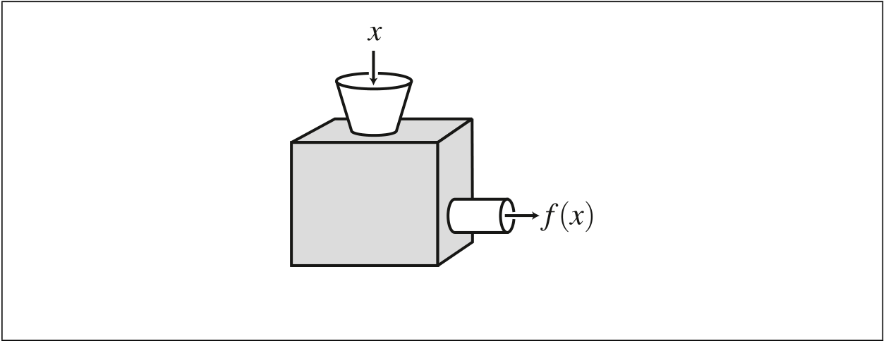
For example, consider the set F = {(n,n2) | n ∈ Z}. The set F is a subset of Z × Z that satisfies the conditions given in Definition 4.1.1, and hence F can be thought
of as defining a function Z → Z. However, the set F is also a subset of Z × R that satisfies the conditions in the definition of a function, and hence F can be thought
certain elements of B, where there is an arrow from a to b when (a,b) is in the subset.
For example, let A = {a,b,c,d} and B = {1,2,3,4}. Two diagrams with arrows from A to B are seen in Figure 4.1.2. In Part (i) of the figure the diagram corresponds to the
4 4
(i) (ii)
tainly do not have a function, because not everyone has a sister. Even if we restrict
the domain to all people with sisters there is a problem, because some people have
| 4.1 Functions | 133 |
|---|---|
properly define a function, because we are not given a domain and codomain. It is (3) Consider the formula f(x) =√x2−5x+6. On its own, this formula does not standard, however, when given a formula such as this to take as its domain the largest subset of R that can serve as a domain; in this case the set (−∞,2] ∪ [3,∞) is taken as the domain. The codomain might as well be taken to be R, though various subsets of R could be taken as the codomain as well, for example [−17,∞). ♦ |
|
| 4.1 Functions | 135 |
|---|---|
The concept of a function being well-defined has a more general meaning than what we stated above. In general, a function is said to be well-defined if there is some potential problem with the definition of the function, and it turns out that the problem does not in fact occur. In practice, saying that a function is well-defined usually means that one of two things has been verified: that every element of the domain is indeed taken into the codomain, or that the function has only one value for every element of the domain. Our use of the term well-defined in the previous paragraph is of the second type. An example of the first type of use of the term well-defined occurs in Exercise 4.4.8. A look at the special case of functions R → R can help us gain some insight into functions generally. Let f : R → R be a function. Then f gives rise to a graph in R2, where the graph consists of all points in R2of the form (x, f(x)), where x ∈ R. For each such x, the definition of functions implies that there is one and only one corresponding value f(x) ∈ R. Hence, for each x ∈ R there is one and only one point on the graph of f that is on the vertical line through x. See Figure 4.1.3. Conversely, suppose that we are given a curve in R2. Is this curve necessarily the graph of some function g: R → R? If the curve has the property that it intersects each vertical line in the plane at precisely one point, then the curve will be the graph of some function a function. g: R → R; if this property does not hold, then the curve will not be the graph of such |
|
As we noted earlier, a function consists of three things: a domain, a codomain and a subset of the product of the domain and the codomain satisfying a certain
Therefore the domain of f is the same as the domain of g.
...
(argumentation)
...Then f(a) = g(a).
2. The identity map on A is the function 1A : A → A defined by 1A(x) = x for all x ∈ A.
3. The inclusion map from S to A is the function j: S → A defined by j(x) = x for all x ∈ S.
| 4.1 Functions | 137 |
|---|---|
(3) We can think of R2as R×R. We then have the two projection maps π1 : R2→R and π2 : R2→ R that are defined by π1((x,y)) = x and π2((x,y)) = y for all (x,y) ∈R2. That is, the projection map π1 picks out the first coordinate of the point (x,y), for all (x,y) ∈ R2, and similarly for π2. ♦ In addition to the general types of functions given in Definition 4.1.3, which we will use throughout this text, we will also make use of some standard functions R → R, such as polynomials, exponentials, logarithms and trigonometric functions in various examples. It is beyond the scope of this text to define these standard func-tions, but they can indeed be defined rigorously, and all the familiar properties can be proved, so no harm is done in our using these functions. See [Blo11, Chapter 7] for rigorous definitions of such functions. |
|
Exercise 4.1.1. Let A = {a,b,c} and B = {1,2,3}. Which of the following subsets of A×B are functions A → B?
138 4 Functions
(1) f(a) is the mother of a.
(2) g(a) is a brother of a.
|
|---|
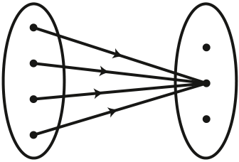
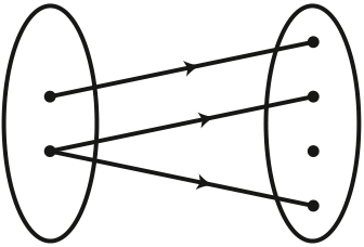
(1) Let f(x) = cosx.
(2) To every person a, let g(a) be the height of a in inches.
Exercise 4.1.9. [Used in Section 4.1.] Restate Theorem 4.1.5 in a non-indexed ver-sion.
the latter in the proof of the former, it will follow that the two results are equivalent. We make use here of the version of the Axiom of Choice stated in Theorem 4.1.5. Let I be a non-empty set, and let {Ai}i∈I be a family of non-empty sets indexed by I. Assume Zorn’s Lemma. We will show that there is a choice function for {Ai}i∈I. (1) A partial choice function for {Ai}i∈I is a function fJ : J →�J ⊆ I such that fJ(j) ∈ A j for all j ∈ J. If fJ is a partial choice function for j∈JAjfor some
(2) Let P be the set of all partial choice functions for {Ai}i∈I, and let C be a chain
We might also want to find all the adults whose heights are at least 6 ft. and no more than 6 ft. 3 in. Because we are working in inches, we therefore want to find all people whose heights are in the interval [72,75]. Hence, we want the set {x ∈ A | h(x) ∈ [72,75]}. In this case we are taking a subset of the codomain, namely, a certain set of possible heights, and finding the corresponding subset of the domain, namely, all people whose heights are as desired.
B, we want to take each subset P of A, and see where f sends all of its elements The following definition generalizes the above process. Given a function f : A →

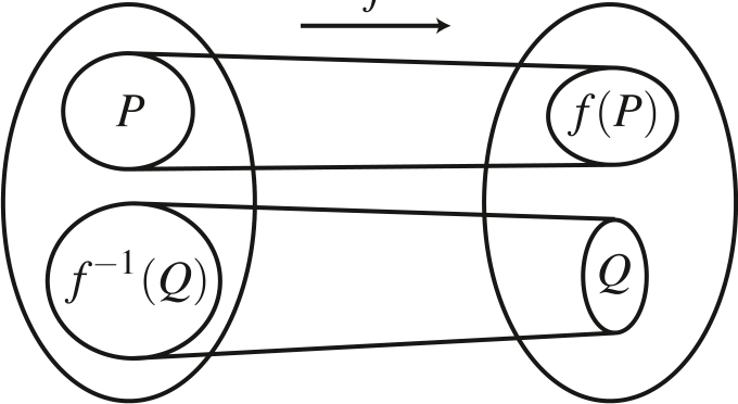
| 4.2 Image and Inverse Image | 141 |
|---|---|
|
|
However, the method of defining these sets given in Definition 4.2.1 will be more useful to us than these alternatives.
The terms “range” and “codomain” are often confused, so precise use of language is needed.
similar to the notation f−1(Q), the concept of an inverse image of a set and the
concept of an inverse function are quite different, and it is the similarity of notation
set Q under f−1, because f−1(Q) is used even in cases where the function f−1does
not exist. Proofs about sets of the form f−1(Q) should not make use of an inverse
Example 4.2.3. Let h: R → R be defined by h(x) = x2for all x ∈ R. It is straightfor-ward to compute that h([0,3]) = [0,9] and h([−2,2]) = [0,4]. Then h−1(h([0,3])) = h−1([0,9]) = [−3,3]. We therefore see that h−1(h([0,3])) ̸= [0,3]. Similarly, we compute that h(h−1([−4,4])) = h([−2,2]) = [0,4], and hence h(h−1([−4,4])) ̸= [−4,4]. ♦
For the proof of the following theorem, as well as for subsequent results involving
sort of thing to which they could be equal), we use the standard strategy for proving
equality of sets, which is showing that each set is a subset of the other.
“x = f(a) for some a ∈ P” can be rewritten as “x ∈ f(P).” Similarly, suppose that we start with a statement of the form “z ∈ f−1(Q).” The definition of f−1(Q) allows us to rewrite the statement as “f(z) ∈ Q,” which again is easier to work with than the original statement. Conversely, a statement of the form “ f(z) ∈ Q” can be rewritten as “z ∈ f−1(Q).” As is the case with many problems in mathematics, going back to the definitions is often the best way to start creating a proof.
The following theorem, the proof of which uses the above mentioned strategies,
| 4.2 Image and Inverse Image | 143 |
|---|---|
subsets of A indexed by I, and let {Vk}k∈K be a family of subsets of B indexed by K.
Proof. We will prove Parts (5) and (6), leaving the rest to the reader in Exercise 4.2.6. 6. f (�7. f (�8. f−1(�9. f−1(�i∈IUi) = �i∈IUi) ⊆ �k∈KVk) = �k∈KVk) = �i∈If(Ui). i∈If(Ui). u ∈ Uj for some j ∈ I. Hence b ∈ f(Uj) ⊆�� �f(v) for some v ∈ Uk. Because v ∈�i∈If(Ui). Next, let a ∈ � i∈IUi) ⊆ ⊓⊔ fact that the function f induces a new function f∗: P(B) → P(A), which is defined by f∗(P) = f−1(Q) for all Q ∈ P(B). From that point of view, the terms “image” and images and inverse images, it is usually more useful in the course of formulating proofs to think of images and inverse images as we have done until now, and so we |
|
(3) Let h: R → (0,∞) be defined by h(x) = ex−1+3 for all x ∈ R. (4) Let p: R → R be defined by p(x) =√x4+5 for all x ∈ R.
(5) Let q: R → [−10,10] be defined by q(x) = sinx+cosx for all x ∈ R.
(4) m−1([−5,3]).
(5) m−1({0}).
Exercise 4.2.3. For each of the following functions f : R → R and each set T ⊆ R, find f(T), f−1(T), f(f−1(T)) and f−1(f(T)).
(2) g−1([−1,1]).
Exercise 4.2.5. Let X and Y be sets, let A ⊆ X and B ⊆ Y be subsets and let π1 : X ×Y → X and π2 : X ×Y → Y be projection maps as defined in Section 4.1.
(9).
Exercise 4.2.7. Find the flaw(s) in the following alleged proof of Theorem 4.2.4 (8),
k∈KVk.
Exercise 4.2.8. In this exercise we show that it is not possible to strengthen Theo-
Exercise 4.2.9. Find an example to show that the “⊆” in Theorem 4.2.4 (7) cannot be replaced with “=.” It is sufficient to use the intersection of two sets.
Exercise 4.2.10.
(1) Prove that f(P)− f(Q) ⊆ f(P−Q).
(2) Is it necessarily the case that f(P − Q) ⊆ f(P) − f(Q)? Give a proof or a counterexample.
Exercise 4.2.12. Let A and B be sets, let C,D ⊆ B be subsets and let f : A → B be a function. Prove that f−1(D−C) = f−1(D)− f−1(C).
(6) Prove that f−1(f(f−1(Y))) = f−1(Y).
Exercise 4.2.14. Let A and B be sets, and let f,g: A → B be functions. Think of these functions as inducing functions f∗,g∗ : P(A) → P(B), and functions f∗,g∗: P(B) →P(A). Prove that f∗ = g∗ if and only if f∗= g∗if and only if f = g.
(2) Prove that there is some T ∈ P(A) such that g(T) = T. Such an element T is called a fixed point of g. Use Part (1) of this exercise.
146 4 Functions
(g◦ f)(x) = g(f(x))
for all x ∈ A. △
because g◦ f means doing f first and then g even though we generally read from left to right in English. Think of “◦” as meaning “following.” We will stick with the “◦”notation in spite of any slight confusion it might cause at first, because it is extremely
widespread, and because the reader will find that it works well once she is used to it.
4.3 Composition and Inverse Functions 147
One way to visualize the composition of functions is to use “commutative dia-grams.” If f : A → B and g: B → C are functions, then we can form g◦ f : A → C, and we can represent all three of these functions in the following diagram.
Definition 4.3.3. Let B be a set, let A1,...,An be sets for some n ∈ N and let f : B → A1 ×···×An be a function. For each i ∈ {1,...,n}, the i-th coordinate function of f, denoted fi, is the function fi : B → Ai defined by fi = πi ◦ f, where πi : A1 ×···×An → Ai is the projection map. △ The fact that fi = πi ◦ f for all i ∈ {1,...,n}, as given in Definition 4.3.3, means that f(x) = (f1(x),..., fn(x)) for all x ∈ B. In some texts this fact is abbreviated by writing f = (f1,..., fn), or alternatively by writing f = f1 × ··· × fn. How-ever, although the notations (f1,..., fn) and f1 × ··· × fn could be formally de-fined to be the function we have denoted f, the reader is urged to use these two notations with caution, or to avoid them at all, for the following reason. Whereas writing f(x) = (f1(x),..., fn(x)) is perfectly sensible, the two sides of the equa-tion being different expressions for the same element of A1 × ··· × An, using the notation f = (f1,..., fn) might mistakenly suggest that the function f is an ele-ment of the product of n sets, which is not necessarily true, and using the notation
also not necessarily true. f = f1 × ··· × fn might mistakenly suggest that f is the product of n sets, which is
Example 4.3.4. Let f : R2→ R3be defined by
f((x,y)) = (xy,sinx2,x+y3)
1. (h◦g)◦ f = h◦(g◦ f) 2. f ◦1A = f and 1B ◦ f = f (Associative Law). (Identity Law).
Proof.
Do functions have inverses under composition? That is, for any given function is there another that “cancels it out” by composition? In arithmetic, for example, we can cancel out the number 3 by adding −3 to it, which yields 0. For functions, the operation addition and the number 0 are replaced with composition of functions and the identity map, respectively. However, the non-commutativity of composition means that we need a bit more care when we define “canceling out” for functions than we do with addition (which is commutative).
Definition 4.3.6. Let A and B be
sets, and let f : A → B and g: B → A
be functions. 1. The function g is a
right inverse for f if f ◦g =
1B.
2. The function g is a left
inverse for f if g◦ f = 1A.
2. If f has a right inverse g and a left inverse h, then g = h, and hence f has an inverse.
3. If g is an inverse of f, then f is an inverse of g.
By the definition of inverses, it follows that f is an inverse of g. (3). Suppose that g: B → A is an inverse of f. Then g ◦ f = 1A and f ◦ g = 1B.⊓⊔
Observe that the proof of Lemma 4.3.7 (1) is virtually identical to the proof of the uniqueness part of Theorem 2.5.2. The same proof in a more generalized setting is also used for Lemma 7.2.4. Lemma 4.3.7 (1) allows us to make the following definition.
We note that if f : A → B has an inverse f−1: B → A, then f−1(f(x)) = x for all x ∈ A and f(f−1(x)) = x for all x ∈ B. Another way of stating the relation between
This latter formulation will not be particularly useful to us in the construction of f and f−1is to say that y = f−1(x) if and only if x = f(y) for all y ∈ A and x ∈ B.
that k has an inverse, the function j:
(3,5) → (0,1) defined by
j(x) =x−3
(1) Let k: (0,1) →
(3,5) be defined by k(x) = 2x+3 for
all x ∈ (0,1). We claim for all x ∈
(3,5). We compute j(k(x))
=(2x+3)−3 = x for all x ∈
(0,1), and hence j ◦ k = 1(0,1). Similarly,
we compute k(j(x)) = 2
·x−3 2+ 3 = x for all x
∈ (3,5), and hence
| Exercises |
|---|
Exercise 4.3.1. For each pair of functions f and g given below, find formulas for
f ◦g and g◦ f (simplifying when possible).
(4) Let f : R → R be defined by f(x) = ⌊x⌋ for all x ∈ R, and let g: R → R be defined by g(x) = ⌈x⌉ for all x ∈ R, where ⌊x⌋ and ⌈x⌉ are respectively the greatest integer less than or equal to x and the least integer greater than or
equal to x.
x, if 0 ≤ x if x < 0.
Exercise 4.3.3. Let f,g: R → R be defined by
(2) Find two functions s,t : R → R
such that s ̸= 1R and t ̸= 1R, but t ◦s = 1R.
Exercise 4.3.5. [Used in Theorem 6.3.11 and Theorem
6.6.5.] Let A and B be sets, let U ⊆
A and V ⊆ C be subsets, and let f : A →
B and g: B → C be functions. Prove that
(g◦ f)−1(V) =
f−1(g−1(V)). (g◦
f)(U) = g(f(U)) and
Exercise 4.3.6. Let A, B and
C be sets, and let f : A → B and g:
B →C be functions. Suppose that f and g have
inverses. Prove that g ◦ f has an inverse, and that (g
◦f)−1= f−1◦g−1.
Exercise 4.3.7. Find two right inverses for each of the following functions.
4.3 Composition and Inverse Functions 153
Exercise 4.3.9. Let h,k: R → R be defined by
Exercise 4.3.10. Let A and B be sets, and let f : A → B be a function. Prove that if f has two distinct left inverses then it has no right inverse, and that if f has two distinct right inverses then it has no left inverse.
Exercise 4.3.11. Let B be a set, let A1,...,Ak be sets for some k ∈ N, let Ui ⊆ Ai be a subset for all i ∈ {1,...,k} and let f : B → A1 ×···×Ak be a function. Prove that
Ai
Exercise 4.3.13. This exercise and the next give examples of definitions of functions by universal property. Rather than defining what a certain function is, we state how it should behave, and then prove that there exists a function satisfying the given be-havior. Such constructions are important in category theory, a branch of mathematics that provides a useful (though abstract) language for many familiar mathematical ideas, and has applications to various aspects of mathematics, logic and computer science. See [AM75] or [Kri81] for an introduction to category theory, and [Pie91] for some uses of category theory in computer science.
Exercise 4.3.14. This exercise is similar to Exercise 4.3.13. Let A, B and C be sets, and let f : A → C and g: B → C be functions. Prove that there exist a set P and functions h: P → A and k: P → B such that f ◦h = g◦k, and that for any set X and functions s: X → A and t : X → B such that f ◦ s = g ◦t, there is a unique function u: X → P such that s = h◦u and t = k ◦u. This last condition is represented by the following commutative diagram. The set P together with the functions h and k are called a pullback of f and g. To define P, consider subsets of A×B.
X
......................................................................................................................................................................................................................................................................... ............ P ................................................................................................................ ............ k B
To understand the criteria for the existence of right inverses and left inverses, we start with an example.
Example 4.4.1. Let P be the set of all people, and let m: P → P be the function that assigns to each person her mother. Does this function have a right inverse or a left inverse? Suppose first that g: P → P is a right inverse for m. That would mean that
It turns out that the two problems identified in Example 4.4.1 are the only obsta-cles to finding right inverses and left inverses, respectively. We now give names to functions that do not have these problems.
Definition 4.4.2. Let A and B be sets, and let f : A → B be a function.
156 4 Functions
tive. Second, we show that k is surjective. Let b ∈ [0,∞). Then k(√b) = (√b)2= b. Hence k is surjective. √x2=�y2= y. Hence k is injec- √b ∈ [0,∞), and so√x2=�y2, of the surjectivity of the function k in Part (1) of this example. The reason h is not injective is because h(−3) = 9 = h(3) even though −3 ̸= 3. (Observe that instead of |
|
|---|---|
| arguments for g and h in Parts (2) and (3) of this example. | ♦ |
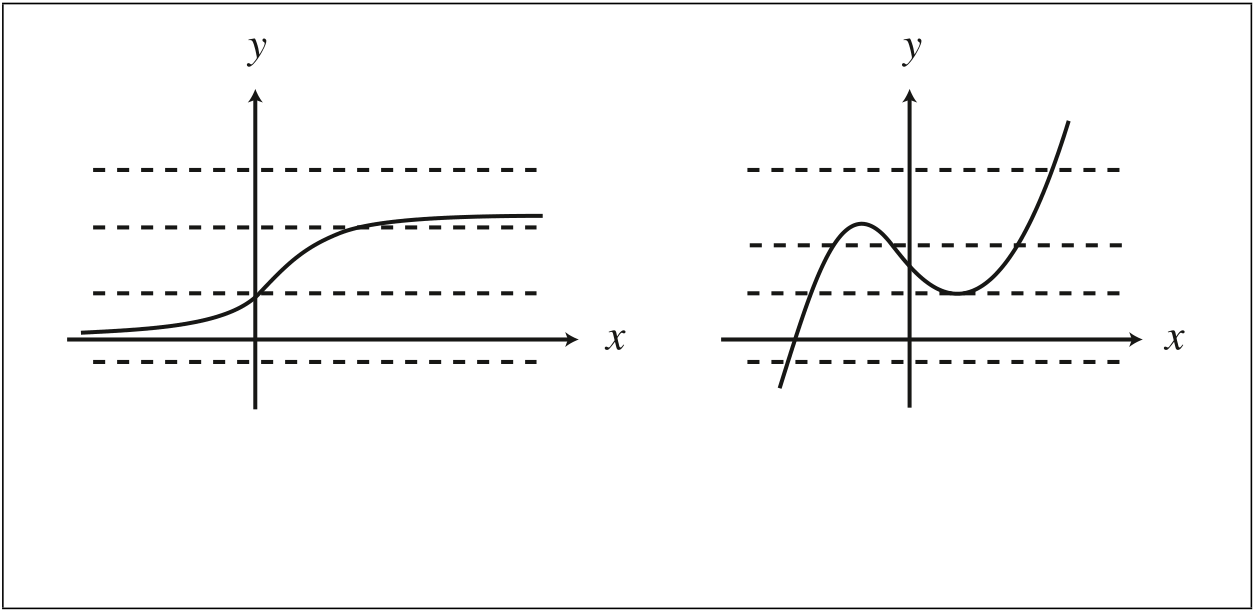
4.4 Injectivity, Surjectivity and Bijectivity 157
Proof. Let x,y ∈ A. Suppose that f(x) = f(y).
...
We will use the above strategies repeatedly, starting with the proof of the follow-ing lemma, which shows that composition of functions behaves nicely with respect to injectivity, surjectivity and bijectivity.
Lemma 4.4.4. Let A, B and C be sets, and let
f : A → B and g: B →C be functions.
1. If f and g are injective, then g◦ f is
injective.
2. If f and g are surjective, then g◦ f is
surjective.
3. If f and g are bijective, then g◦ f is
bijective.
Proof.
The following theorem, which is extremely useful throughout mathematics (and is perhaps the author’s favorite theorem in this text), answers the question posed at the start of this section concerning criteria for the existence of inverse functions.
Theorem 4.4.5. Let A and B be non-empty sets,
and let f : A → B be a function. 1. The
function f has a right inverse if and only if f is
surjective.
2. The function f has a left inverse if and only if
f is injective.
which means that we need to find a function h: B → A such that f ◦ h = 1B. We define h as follows. For each b ∈ B, the surjectivity of f implies that there is at least one element a ∈ A such that f(a) = b; let h(b) = a for some choice of such a (it doesn’t matter which one). It is now true by definition that f(h(b)) = b for all b ∈ B. Hence f ◦h = 1B.
(2). Left to the reader in Exercise 4.4.9.
for the sake of brevity and in order to avoid distraction from the essential idea of the
proof of Theorem 4.4.5, we did not explicitly make use of the Axiom of Choice in
of Choice or something equivalent, but it turns out that that would not have been pos-
sible, because Theorem 4.4.5 (1) is in fact equivalent to the Axiom of Choice, as seen
Theorem 4.4.6. Let A and B be non-empty sets, and let f : A → B be a function.
1. The function f is injective if and only if f ◦ g = f ◦ h implies g = h for all functions g,h: Y → A for all sets Y.
| 160 |
|
|---|---|
q: B → A. Then (g ◦ f) ◦ q = (h ◦ f) ◦ q. Using Lemma 4.3.5 and the definition of right inverses, it follows that g◦(f ◦q) = h◦(f ◦q), and hence g◦1B = h◦1B, and therefore g = h. |
|
(3) Let g: [0,∞) → [0,1) be defined by g(x) =
(4) Let k: R2→ R be defined by k((x,y)) = x2+y2for all (x,y) ∈ R2.(5) Let Q: N → P(N) be defined by Q(n) = {1,2,...,n} for all n ∈ N.
x2 |
|
Prove that f is bijective. Use only the methods we have used in this text, including the standard algebraic properties of the real numbers; do not use calculus.
Exercise 4.4.5. Let A and B be sets. Prove that there is a bijective function f : A×B →B×A.
Exercise 4.4.6. [Used in Section 3.3.] Let A, B and C be sets. Prove that there is a bijective function g: (A×B)×C → A×(B×C).
(2) Prove that U((a,b)) ̸= (a,b) and D((a,b)) ̸= (a,b) for all (a,b) ∈ L. (3) Prove that U and D are injective.
(4) Prove that U(L)∩D(L) = /0.
Exercise 4.4.12. Let A and B be sets, and let f : A → B be a function.
(1) Prove that f is injective if and only if E = f−1(f(E)) for all subsets E ⊆ A.
162 4 Functions
Exercise 4.4.14. [Used in Section 4.4.] Let A, B and C be sets, and let f : A → B and g: B → C be functions.
this exercise are the best possible results.
Exercise 4.4.15. [Used in Theorem 4.4.6.] Prove Theorem 4.4.6 (1).
(4) Prove that f∗is surjective if and only if f is injective.
(5) Prove that f∗ is bijective if and only if f∗is bijective if and only if f is
is sufficient to prove the Axiom of Choice for Pairwise Disjoint Sets. Although Ex-
ercise 3.5.2 was stated for the family of sets versions of the Axiom of Choice, that
Theorem 4.1.5), and make use of that version in this exercise.
Exercise 4.4.20. [Used in Exercise 4.4.21.] Let A be a non-empty set, and let f : A →A be a function. Suppose that f is bijective. For each n ∈ N, let fndenote the function A → A given by fn= f ◦···◦ f .
For each n ∈ N, let f−n= (fn)−1. It can be verified that fa◦ fb= fa+band (fa)b=
part of this exercise; the interested reader can find the details of the first of these fabfor all a,b ∈ Z, though we omit the details for the sake of getting to the interesting
c. If y = fn(x) for some n ∈ Z, and z = fm(y) for some m ∈ Z, then z =
(In Section 5.3 we will see that these three properties are particularly impor-fp(x) for some p ∈ Z.
Putting these observations together, we see that A can be broken up into dis-d. A =�x∈AOx.
joint sets, each of which is the orbit of all its members. (Using the terminol-
(1) Prove that fm= 1A for some m ∈ N. Use the fact that because A is finite, there are only finitely many bijective functions A → A; this fact is proved in Theorem 7.7.4 (3). Let r ∈ N be the smallest natural number such that fr= 1A. (It makes sense intuitively that there is such a smallest natural number;
formally we make use of the Well-Ordering Principle (Theorem 6.2.5).)
164 4 Functions
(7) Prove that nx|r.
(12) For each m ∈ {0,...,r−1}, the fixed set of m, denoted Am, is the set defined by Am = {z ∈ A | fm(z) = z}. Prove that r · B = ∑r−1 special case of Burnside’s Formula; see [Fra03, Section 17] for details. i=0|Ai|. This result is a
4.5 Sets of Functions
will use sets of functions briefly at the end of Section 6.7, and a bit more exten-
sively in Section 7.7. The material in this section is among the most conceptually
For any set A and B, we observe that F (A,B) is also a set, where each element of
the set F (A,B) is a function A → B. There is no theoretical problem with having a set that has elements that are functions, though sometimes it is hard to get an intuitive
(1) If A ̸= /0 and B = /0, then F (A,B) = /0. If A = /0, then F (A,B) = {/0}. If A ̸= /0 and B ̸= /0, then F (A,B) ̸= /0, because there is at least one constant map A → B. (2) Let A = {1,2} and B = {x,y}. Then F (A,B) = {f,g,h,k}, where the func-tions f,g,h,k: A → B are defined by f(1) = x and f(2) = x, by g(1) = x and g(2) = y, by h(1) = y and h(2) = x, and by k(1) = y and k(2) = y.
(3) The set F (R,R) has a number of useful subsets, including the set C(R,R) of
(4) We can give an intuitive interpretation of the set F (N,R) as follows. Let
f ∈ F (N,R). Then we obtain a sequence of real numbers by writing f(1), f(2), f(3), .... Conversely, given a sequence of real numbers a1, a2, a3, ..., we can define
we give two typical results. We start with a relatively simple lemma, which will be
of use later on.
A ......................................................................................................................................... ............ h B
f ..................................................................................................................................................... ..................................................................................................................................................... g
The theorem says that there is a bijective function from P(A) to F (A,{0,1}). What, intuitively, is the relation between elements of P(A), each of which is a subset of A,
and elements of F (A,{0,1}), each of which is a function A → {0,1}? Let S ∈ P(A), so that S ⊆ A. We want to associate with this set S a function A → {0,1}. To do so, observe that we can divide A into the two disjoint subsets S and A−S. We then define a function from A to {0,1} by assigning the value of 1 to every element in S, and 0 to
Theorem 4.5.4. Let A be a set. Then there is a bijective function from P(A) to
F (A,{0,1}).
surjective, starting with the former. Let S,T ∈ P(A). Suppose that Φ(S) = Φ(T). Then χS = χT, and it follows from Exercise 4.1.8 that S = T. Therefore Φ is injective.
We now show that Φ is surjective. Let f ∈ F (A,{0,1}). Let S = f−1({1}), so that S ∈ P(A). We will show that Φ(S) = f, which is the same as showing that χS = f. Both χS and f are functions A → {0,1}. Observe that A − S = f−1({0}). Then, if y ∈ A, we see that
=�1,
0,
if f(y) = 1
Ψ ◦Φ = 1P(A) and Φ ◦Ψ = 1F (A,{0,1}).
Let S ∈ P(A). Then
| 4.5 Sets of Functions | 167 ⊓⊔ |
||
|---|---|---|---|
| χ f −1({1})(y) = |
|
||
| = |
|
||
(1) Let A and B be the sets given in Example 4.5.2 (2). It is seen that B(A,B) = I(A,B) = {g,h}.
show in Exercise 4.5.8, it turns out that I(A,C) has six elements. This example is a (2) Let A = {1,2} and C = {x,y,z}. Then B(A,C) = /0. As the reader is asked to
element f(1) is the first element in the ordered pair, and f(2) is the second element in the ordered pair. Hence the product A×B can be thought of as the set of functions
{ f ∈ F ({1,2},A∪B) | f(1) ∈ A and f(2) ∈ B}.
Choice, and that is what looks so familiar in Definition 4.5.7. If the reader compares the statement of the Axiom of Choice given in Theorem 4.1.5 with Definition 4.5.7, it is immediately evident that not only does the Axiom of Choice imply the following theorem, but the following theorem implies the Axiom of Choice; that is, the Axiom of Choice and the following theorem are equivalent.
Theorem 4.5.8. Let I be a non-empty set, and let {Ai}i∈I be a family of non-empty sets indexed by I. Then ∏i∈I Ai ̸= /0.
| Exercise 4.5.1. Let X = {l,m,n} and Y = {α,β}. Describe all the elements of F (X,Y). |
|---|
(1) Prove that F (C,A) ⊆ F (C,B).
(2) Prove that there is an injective function F (A,C) → F (B,C).
Exercise 4.5.7. Let A be a set, and let g: A → A be a function. Suppose that g is bijective.
(1) Let Ωg : F (A,A) → F (A,A) be defined by Ωg(f) = g◦ f for all f ∈ F (A,A). Prove that Ωg is bijective.
(2) Prove that there is a bijective function from B(A,B) to B(C,D).
Exercise 4.5.10. [Used in Theorem 7.7.4 and Theorem 7.7.12.] Let A and B be sets,
Exercise 4.5.11. Let A be a set. Let Φ : B(A,A) → B(A,A) be defined by Φ(f) = f−1for all f ∈ B(A). Prove that Φ is bijective.
Exercise 4.5.12. Let A be a set. A Z-action on A is a function Γ : Z → B(A,A) that satisfies the following two properties: (1) Γ (0) = 1A, and (2) Γ (a+b) = Γ (a)◦Γ (b) for all a,b ∈ Z.
Mathematicians do not study objects, but relations between objects.
– Henri Poincar´e (1854–1912)5.1 Relations
Undergraduate Texts in Mathematics, DOI 10.1007/978-1-4419-7127-2_5,
© Springer Science+Business Media, LLC 2011
{(1,y),(1,z),(2,y)}. Then 1 E y, and 1 E z, and 2 E y, but 3 ̸E x. (2) Let P be the set of all people. Define a relation on P by having person x related to person y if and only if x and y have at least one parent in common. (3) The symbols < and ≤ both represent relations on R. (4) Let P be the set of all people, and let B be the set of all books. Define a relation from P to B by having person x related to book b if and only if x has read b. (5) Let A be a set. The symbol “⊆” represents a relation on P(A), where P,Q ∈P(A) are related if and only if P ⊆ Q.
a certain condition. Hence f is also a relation from A to B. The concept of a relation (6) Let f : A → B be a function. Then f is defined by a subset of A×B satisfying
Then x S y.
Second, suppose that x S y.
...
Just as a person might wish to find out who all of her relatives are, if we have a relation from a set A to a set B, it is sometimes useful to find all the elements of B that are related to a given element in A.
Definition 5.1.3. Let A and B be non-empty sets, let R be a relation from A to B, and let x ∈ A. The relation class of x with respect to R, denoted R[x], is the set defined by
R[x] = {y ∈ B | x R y}.
In the following definition we give three such properties of relations that will be useful to us in the next two sections, and in many parts of mathematics.
Definition 5.1.5. Let A be a non-empty set, and let R be a relation on A.
Example 5.1.6.
(1) The relation of congruence of triangles in the plane is reflexive, symmetric and transitive.
(7) The relation < on R is transitive, but neither reflexive nor symmetric. Let x,y,z ∈ R. The relation is transitive, because if x,y,z ∈ R, and if x < y and y < z, then x < z. The relation is not reflexive, because it is never the case that x < x, for any x ∈ R. (Observe that we have much more here than the minimum needed to prove that the relation < is not reflexive; it would have sufficed to know that z ≮ z for a single z ∈ R.) The relation is not symmetric, because if x,y ∈ R, and x < y, it is never the case that y < x. (Again, we have much more than is minimally needed to prove that < is not symmetric.)
(8) The relation of one person being the daughter of another person is neither reflexive, symmetric nor transitive. ♦There are standard proof strategies for proving that a relation is reflexive, sym-metric or transitive. Let A be a non-empty set, and let R be a relation on A.
(argumentation)
...Then x R x. Hence R is reflexive. ⊓⊔ If we wish to prove that R is symmetric, we need to show that x R y implies y R x for every x,y ∈ A. Observe that to prove that R is symmetric, we do not prove that
| 5.1 Relations | 175 |
|---|---|
|
|
|
⊓⊔ |
| ⊓⊔ | |
Exercise 5.1.1. For each of the following relations on Z, find the relation classes [3] and [−3] and [6].
(1) Let S be the relation defined by a S b if and only if a = |b|, for all a,b ∈ Z.
(3) Let Z be the relation defined by (x,y) Z (z,w) if and only if x = z or y = w, w2, for all (x,y),(z,w) ∈ R2.
for all (x,y),(z,w) ∈ R2.
(4)¯P = {(1,1),(2,2),(3,3)}.
(5)¯Q = {(1,2),(2,1),(1,3),(3,1),(1,1)}.
(1) Let S be the relation on R defined by x S y if and only if x = |y|, for all x,y ∈ R. (2) Let P be the set of all people, and let R be the relation on P defined by x R y
(3) Let T be the set of all triangles in the plane, and let G be the relation on T if and only if x and y were not born in the same city, for all x,y ∈ P.
(6) Let D be the relation on N defined by a D b if and only if a|b, for all a,b ∈ N.
(7) Let T be the relation on Z × Z defined by (x,y) T (z,w) if and only if there is a line in R2that contains (x,y) and (z,w) and has slope an integer, for all
essarily either?
(2) If R symmetric, is R′necessarily symmetric, necessarily not symmetric or not
metric and transitive. Find the flaw in the following alleged proof that this relation is
necessarily reflexive; there must be a flaw by Example 5.1.6 (4). “Let x ∈ A. Choose
x,y ∈ A.
(3) Suppose that R is transitive. Prove that if x R y, then [y] ⊆ [x], for all x,y ∈ A.
(4) Let k: R2→ R be defined by k((x,y)) = 3x2+6xy+3y2for all (x,y) ∈ R2; let M be the relation on R2defined by (x,y) M (z,w) if and only if x+y = z+w, for all (x,y),(z,w) ∈ R2.
Exercise 5.1.10. Let A and B be sets, let R be a relation on A and let f : A → B be a function. Suppose that f is injective, and that it respects the relation R, as defined in Exercise 5.1.9. What, if anything, can be proved about the relation R?
In this section we discuss a very important type of relation on the set of integers, which will serve to illustrate the general topic discussed in the next section, and is also a valuable tool in various parts of mathematics and its applications, for example number theory, cryptography and calendars. See [Ros05, Chapters 4 and 5] for fur-ther discussion of congruence and its applications, and see [Kob87] for a treatment of congruence and cryptography.
The idea of congruence is based upon the notion of “clock arithmetic,” a term sometimes used in elementary mathematics. (For the reader who has not seen “clock arithmetic,” it will be sufficient to have seen a clock). For the sake of uniformity, we will make all references to time using the American 12-hour system (ignoring a.m. vs. p.m.), as opposed to the 24-hour system used many places around the world, and in the U.S. military.
Definition 5.2.1. Let n ∈ N, and let a,b ∈ Z. The number a is congruent to the number b modulo n, denoted a ≡ b (mod n), if a−b = kn for some k ∈ Z. △Example 5.2.2. We see that 19 ≡ −5 (mod 4), because 19−(−5) = 24 = 6·4; and 7 ≡ 7 (mod 3), because 7−7 = 0 = 0·3; and 13 ̸≡ 2 (mod 9), because 13−2 = 11 and 11 is not a multiple of 9. ♦
following lemma shows that for each n, this relation is reflexive, symmetric and For each n ∈ N, we obtain a relation on Z given by congruence modulo n. The
3. If a ≡ b (mod n) and b ≡ c (mod n), then a ≡ c (mod n). Proof.
(1). Observe that a−a = 0·n.
this theorem makes use of an important fact about the integers known as the Division
Algorithm, which is stated as Theorem A.5 in the Appendix.
Corollary 5.2.5. Let n ∈ N, and let a ∈ Z. Then precisely one of the following holds: either a = nk for some k ∈ Z, or a = nk +1 for some k ∈ Z, or a = nk +2 for some k ∈ Z, ..., or a = nk +(n−1) for some k ∈ Z.
If we use n = 2 in Corollary 5.2.5, we deduce the following familiar result.
...
[0] = {...,−10,−5,0,5,10,...}
[5] = {...,−5,0,5,10,15...}.
...
tinct classes. Moreover, these classes are disjoint, and their union is all of Z. The
analogous result holds for arbitrary n, as stated in the following theorem.
(1). Suppose that a ≡ b (mod n). Let x ∈ [a]. Then by the definition of relation classes we know that a ≡ x (mod n). By Lemma 5.2.3 (2) it follows that b ≡ a (mod n), and hence by Lemma 5.2.3 (3) we deduce that b ≡ x (mod n). Therefore x ∈ [b], and hence [a] ⊆ [b]. A similar argument shows that [b] ⊆ [a]. We conclude that [a] = [b].
Now assume that a ̸≡ b (mod n). We use proof by contradiction. Suppose that [a]∩[b] ̸= /0. Hence there is some y ∈ [a]∩[b]. Then y ∈ [a] and y ∈ [b], so that a ≡ y (mod n) and b ≡ y (mod n). By Lemma 5.2.3 (2) we see that y ≡ b (mod n), and by Lemma 5.2.3 (3) it follows that a ≡ b (mod n), which is a contradiction. We conclude that [a]∩[b] = /0.
Definition 5.2.8. Let n ∈ N. The set of integers modulo n, denoted Zn, is the set defined by Zn = {[0],[1],...,[n−1]}, where the relation classes are for congruence modulo n. △
The set Zn is also denoted Z/nZ in some texts, for reasons that will become
so Z12 = {[12],[1],...,[11]}, which is what we see on the face of a clock. For math-ematical purposes it is more convenient to write [0] rather than [12], and so we will
continue to write Z12 as we did originally; it would also be nice to have the 12 on
are many sets with n elements, but what makes Zn particularly useful is that there For each n ∈ N, the set Zn has n elements. Of course, for each n ∈ N, there
is a natural way to define addition and multiplication on it, as seen in the follow-
Definition 5.2.10. Let n ∈ N. Let + and · be the binary operations on Zn defined by [a]+[b] = [a+b] and [a]·[b] = [ab] for all [a],[b] ∈ Zn. △
As reasonable as Definition 5.2.10 seems, there is a potential problem. Let n ∈N, and let [a],[b],[c],[d] ∈ Zn. Suppose that [a] = [c] and [b] = [d]. Do [a+b] = [c+d] and [ab] = [cd] necessarily hold? If not, then we could not say that [a] +
we verify using the following lemma.
Lemma 5.2.11. Let n ∈ N, and let a,b,c,d ∈ Z. Suppose that a ≡ c (mod n) and b ≡ d (mod n). Then a+b ≡ c+d (mod n) and ab ≡ cd (mod n).
From Lemma 5.2.11, together with Theorem 5.2.7 (1), we deduce the following
corollary, which we state without proof. This corollary tells us that + and · as given in Definition 5.2.10 are indeed well-defined for each Zn.
182 5 Relations
(See Section 7.1 for more discussion of such operation tables.) Consider the follow-
| [0] [1] [2] [3] [4] [5] | |
|---|---|
| [0] [1] [2] [3] [4] [5] |
[0] [1] [2] [3] [4] [5] [1] [2] [3] [4] [5] [0] [2] [3] [4] [5] [0] [1] [3] [4] [5] [0] [1] [2] [4] [5] [0] [1] [2] [3] [5] [0] [1] [2] [3] [4] |
the form ax = b, always has a unique solution whenever a ̸= 0. The situation in Zn is more complicated. Consider the equation [4] · x = [3]. In Z11 there is a unique solution, which is x = [9], as can be verified simply by trying each element of Z11 as a possible candidate for x. In Z12 the same equation has no solution, as can again be verified by trying each element of Z12. The equation [3]·x = [0] has three solutions in Z6, which are x = [0],[2],[4], as can be seen using the operation table for · for Z6. We therefore see that in Z6 it is possible to have two non-zero elements such that their product is [0], in contrast to the situation for multiplication of real numbers. See [Fra03, Section 20] for further discussion of this type of equation in Zn.
Our final comment about Zn takes us back to our initial discussion of clocks, where we took the number 41 (which was the result of starting at 11 o’clock and adding 30 hours), and we then subtracted the number 12 as many times as needed from 41 until a number in the 1 to 12 range was obtained; in this case we obtained the number 5. There are, of course, infinitely many numbers in Z that, when treated in this same way, will yield the number 5. Rather than thinking of the number 5 here as an integer, it is more correct to think of it as an element of Z12. That is, we think of taking infinitely many elements of Z, and we send them all to a single element in Z12. Of course, there is nothing special about the number 5, and there is nothing special about working modulo 12. We now use functions to formalize this process.
ical map that will be seen in Definition 5.3.8. The canonical map γ : Z → Zn is a special case of a more general type of canon-
We now see two simple results about the canonical map that are examples of more general, though rather different, phenomena we will see subsequently.
γ ................................................................................................... ..........................................................................................................................................................................................................................................
Zn
In contrast to Lemma 5.2.14, which can be generalized to all equivalence re-lations, as seen in Lemma 5.3.9, the following property of the canonical map for congruence modulo n is not applicable to most equivalence relations, though it can be generalized in a very different way, as discussed in Section 7.3.
| Proof. Left to the reader in Exercise 5.2.11. | ⊓⊔ |
|---|
Exercise 5.2.2. Solve each of the following equations in the given set Zn. (In some cases there is no solution.)
184 5 Relations
Exercise 5.2.4. Let n,q ∈ N, and let a,b ∈ Z. Suppose that a ≡ b (mod n), and that q|n. Prove that a ≡ b (mod q).
Exercise 5.2.5. Let n ∈ N, and let a,b ∈ Z. Suppose that a ≡ b (mod n). Prove that n|a if and only if n|b.
the “···” are avoided.
prime number. The converse to this result, known as Wilson’s Theorem, is also true, Let n ∈ N. Suppose that n > 1, and that (n−1)! ≡ −1 (mod n). Prove that n is a
Exercise 5.2.10. [Used in Lemma 5.2.14.] Prove Lemma 5.2.14.
Exercise 5.2.11. [Used in Lemma 5.2.15.] Prove Lemma 5.2.15.
You may use the fact that the statement of Lemma 5.2.11 can be extended to sums
and products of any finite number of integers.
(3) Let ¯Σ(a) be an abbreviation for ΣM(a)(a); that is, the number ¯Σ(a) is the result of repeatedly adding the digits of the number a until a single digit remains. (This process is used in gematria, a method employed in Jewish mysticism, as well as in similar constructions in Greek and Arab traditions; see [Ifr85, Chapter 21] for details.) Does ¯Σ(a + b) =¯Σ(a) +¯Σ(b) always hold? Give a proof or a counterexample. Does ¯Σ(ab) =¯Σ(a) ·¯Σ(b) always hold? Give a proof or a counterexample.
(4) Prove that ¯Σ(a+b) =¯Σ(¯Σ(a)+¯Σ(b)) and ¯Σ(ab) =¯Σ(¯Σ(a)·¯Σ(b)).
Definition 5.3.3. Let A be a non-empty set, and let ∼ be an equivalence relation on A. The relation classes of A with respect to ∼ are called equivalence classes. △ For the rest of this section, in order to avoid trivial cases, we will restrict our attention to non-empty sets. We start with the following theorem, which generalizes
186 5 Relations
cise 5.3.6.
By reflexivity we see that q ∼ q, and therefore q ∈ [q] ⊆�We conclude that�(2). By definition [x] ⊆ A for all x ∈ A, and hence�
The following corollary is derived immediately from Theorem 5.3.4 (1).
Corollary 5.3.5. Let A be a non-empty set, let ∼ be an equivalence relation on A and let x,y ∈ A. Then [x] = [y] if and only if x ∼ y.
at another way, each equivalence class is named after each of its elements, so that a
single equivalence class may have many names, but it is still a single set, and a single
In the following definition, which generalizes Definition 5.2.13, we use functions
to relate a set and its quotient set.
Using the terminology of Exercise 5.1.9, we say that the function f in Lemma 5.3.9
respects ∼. The condition f = g◦γ in Lemma 5.2.14 is represented by the following commutative diagram (as discussed in Section 4.3).
Suppose that we have a quotient set A/∼. We see from Theorem 5.3.4 that any two distinct equivalence classes in A/∼ are disjoint, and that the union of all the equivalence classes is the original set A. We can therefore think of A/∼ as the result of breaking up the set A into disjoint subsets. The following definition generalizes
this notion of breaking up a set into disjoint subsets.
| △ |
|---|
188 5 Relations
Definition 5.3.10 (a) can be rephrased more concisely by saying that D is pair-wise disjoint, using the terminology of Definition 3.5.1, though here we use the non-indexed version of the definition. A schematic representation of a partition of a set is seen in Figure 5.3.1. Another way of looking at partitions is to observe that if E is a family of subsets of a set A, then E is a partition of A if and only if for each x ∈ A, there is one and only one P ∈ E such that x ∈ P.
(2) Let C = {[n,n+1)}n∈Z. Then C is a partition of R.
(3) Let G = {(n−1,n+1)}n∈Z. Then G is not a partition of R, because it is not pairwise disjoint. For example, we observe that (1−1,1+1) ∩ (2−1,2+1) = (1,2). ♦
using bijective functions. To state our result, we will need the following definition,
which takes us to one higher level of abstraction than we have seen until now in our
TA are. Each element of E(A) is an equivalence relation on A, which formally is a
subset of A×A that satisfies certain conditions. Each element of TA is a partition of A, which is a family of subsets of A that satisfy certain conditions.
¯R1 = {(1,1),(2,2),(3,3)},
¯R2 = {(1,1),(2,2),(3,3),(1,2),(2,1)},
¯R3 = {(1,1),(2,2),(3,3),(1,3),(3,1)},
¯R4 = {(1,1),(2,2),(3,3),(2,3),(3,2)},
¯R5 = {(1,1),(2,2),(3,3),(1,2),(2,1),(1,3),(3,1),(2,3),(3,2)}.
It is straightforward to verify that each of the relations Ri listed above is an equiva-
partitions of A. To state this correspondence precisely, we start by defining, for each
non-empty set A, a function from E(A) to TA, and a function in the other direction. It
non-empty set A, but to avoid unnecessarily cumbersome notation (such as ΦA and
ΨA), we will assume that the set A is always known from the context.
these claims follows immediately from the definition of Φ and Corollary 5.3.12. The
second claim is left to the reader in Exercise 5.3.11. ⊓⊔
in Example 5.3.14. It can be verified that Φ(Ri) = Di and Ψ(Di) =Ri for all i ∈{1,...,5}; details are left to the reader. ♦
In Example 5.3.17 (3), we see that Φ and Ψ are inverses of each other. Quite
relation on A there corresponds a unique partition of A, and vice versa. Moreover, not
only do we know in principle that there is such a correspondence, but, even better,
Proof. We need to show that
| 5.3 Equivalence Relations | 191 |
|---|---|
Let B ∈ F . Then by the definition of Φ we know that B is an equivalence class of≎, so that B = [z] for some z ∈ A. Because B is a partition of A, then there is a unique P ∈ B such z ∈ P. Let w ∈ A. Then by the definition of Ψ we see that z ≎ w if and only if w ∈ P. It follows that w ∈ [z] if and only if w ∈ P, and hence P = [z]. Hence B = [z] = P ∈ B. Therefore F ⊆ B.
|
|
(4) Let P be the set of all people, and let Z be the relation on P defined by x Z y x,y ∈ R.
(5) Let P be the set of all people, and let R be the relation on P defined by x R y if and only if x and y are first cousins, for all x,y ∈ P.
(1) Let R be the relation defined by a R b if and only if |a| = |b|, for all a,b ∈ R.
(2) Let S be the relation defined by a S b if and only if sina = sinb, for all a,b ∈ R.
(1) Let Q be the relation defined by (x,y) Q (z,w) if and only if x2+y2= z2+w2,
for all (x,y),(z,w) ∈ R2.
Exercise 5.3.4. Let A and B be sets, and let f : A → B be a function. Let ∼ be the relation on A defined by x ∼ y if and only if f(x) = f(y), for all x,y ∈ A.
(1) Prove that ∼ is an equivalence relation.
Exercise 5.3.6. [Used in Theorem 5.3.4.] Prove Theorem 5.3.4 (1).
Exercise 5.3.7. [Used in Lemma 5.3.9.] Prove Lemma 5.3.9.
sponding partition. Your description of each partition should have no redundancy,
and should not refer to the name of the relation.
l1 ≏ l2 if and only if l1 is parallel to l2 or is equal to l2, for all l1,l2 ∈ L.
Exercise 5.3.10. For each of the following partitions, describe the corresponding
origin (the origin is considered a “degenerate” circle).
(4) Let W be the partition of R defined by W = {[n,n+2) | n is an even integer}.
(2) Let γ : X → X/≍ be the canonical map. Let j: h(X) → Y be the inclusion map. Prove that there is a unique bijective function ˆh: X/≍ → h(X) such that h = j ◦ˆh◦γ. This last condition is represented by the following commutative diagram (as discussed in Section 4.3).
f
Observe that γ is surjective (because ≍ is reflexive), that ˆh is bijective and that j is injective. Hence any function can be written as a composition of a
surjective function, a bijective function and an injective function.
(4) Suppose that A is a finite set. Express |R (A)| and |SA| in terms of |A|. Do R (A) and SA have the same number of elements? Use Example 3.2.9 (2) and
Example 3.3.10 (3).
(1) Find a set B and an element D ∈ SB such that�(2) Suppose that A is finite and has at least two elements. Prove that each of�Φ set C and an element E ∈ SC such that� and� Ψ(E) is not transitive.
Ψ(D) is not reflexive. Find a
194 5 Relations
These are among the marvels that surpass the bounds of our imagination, and that must warn us how gravely one errs in trying to reason about infinites by using the same attributes that we apply to finites.
– Galileo Galilei (1564–1642)
Undergraduate Texts in Mathematics, DOI 10.1007/978-1-4419-7127-2_6, © Springer Science+Business Media, LLC 2011
196 6 Finite Sets and Infinite Sets
The Peano Postulates for the natural numbers are based on the insight that the most fundamental property of the natural numbers is the ability to do proof by in-duction. Although it might seem that in order to do proof by induction it would also be necessary to be able to do other things with the natural numbers such as addition, it turns out that very little indeed is needed to do proof by induction. We need to have a set, denoted N; we need to have a distinguished element in the set, denoted 1, with which to start proof by induction; and we need to have a function from the set
6.2 Properties of the Natural Numbers 197
If we think intuitively of the function s in the Peano Postulates as taking each natural number to its successor, then Part (a) of the postulates says that 1 is the first number in N, because it is not the successor of anything.
Although it does not say in the Peano Postulates (Axiom 6.2.1) that the set N is unique, in fact that turns out to be true. See [Blo11, Exercise 1.2.8] for a proof. We can therefore make the following definition.
If one goes through the full development of the natural numbers starting from the Peano Postulates, the first major theorem one encounters is the one we now state. This theorem is used in particular in the definition of addition and multiplication of the natural numbers, and although we will not go over those definitions (see the reference given above), this theorem has many other applications in many parts of mathematics. This theorem, called Definition by Recursion, is in fact so valuable that it merits a section of its own, Section 6.4.
Definition by Recursion allows us to define functions with domain N by defining a function at 1, and then defining it at n+1 in terms of the definition of the function at n. It is important to recognize that recursion, while intimately related to induction, is not the same as induction (though it is sometimes mistakenly thought to be); the essential difference is that induction is used to prove statements about things that are already defined, whereas recursion is used to define things. The proof of the follow-ing theorem, which relies upon nothing but the Peano Postulates (Axiom 6.2.1), is somewhat tricky; see [Blo11, Theorem 2.5.5] for details.
f ............................................................................................................................ ............................................................................................................................ f
H ................................................................................................................ ............ H
k
1. If a+c = b+c, then a = b.
2. (a+b)+c = a+(b+c).
8. c(a+b) = ca+cb.
9. (ab)c = a(bc).
14. a < b if and only if a+c < b+c. b ≤ c, then a < c; if a ≤ b and b ≤ c, then a ≤ c.
15. a < b if and only if ac < bc.
20. a < b if and only if a+1 ≤ b.
21. If a < b, there is a unique p ∈ N such that a+ p = b.
The hard part of the proof of the Well-Ordering Principle (Theorem 6.2.5) is the
existence of the number m given in the statement of the theorem; the uniqueness is
that writing “...” alone is not rigorous, except when we give it a rigorous meaning
in specific cases, such as the following.
| and | △ | ||
|---|---|---|---|
selves to write the nonsensical expression “{1,...,0},” and it should be interpreted as the empty set. For the exercises in this section, the reader should use only the properties of the natural numbers stated in this section. Subsequently, the reader should feel free to use any standard properties of the natural numbers, as we have done until now. For the rest of this chapter, we will at times refer to some of the properties of the natural numbers stated in this section to emphasize their role in various proofs. |
|||
Exercise 6.2.4. [Used in Theorem 6.4.5.] Let H be a non-empty set, let a,b ∈ H and let p: H ×H → H be a function. Prove that there is a unique function g: N → H such that g(1) = a, that g(s(1)) = b and that g(s(s(n))) = p((g(n),g(s(n)))) for all
n ∈ N. The main step of the proof is to apply Definition by Recursion (Theorem 6.2.3)
Mathematical induction is a very useful method of proving certain types of state-ments that involve the natural numbers. It is quite distinct from the informal concept of “inductive reasoning,” which refers to the process of going from specific exam-ples to more general statements, and which is not restricted to mathematics. When we use the phrase “proof by induction” we will always refer to the mathematical sort of induction, not this other use of the term.
More precisely, mathematical induction is a method that can be used
to prove able n that is a natural number. For example, we will
shortly prove that the statement statements of the form (∀n ∈
N)(P(n)), where P(n) is a statement
with a free vari-P(n) = “8n− 3nis
divisible by 5” is true for all natural numbers n. How you
origi-nally thought of trying to prove such a statement might have
occurred in many ways, one of which is by playing around with various
numerical examples, for example looking at 81− 31, at
82− 32, and at 83− 33, and then using informal
“inductive reasoning” to conjecture that 8n− 3nis
divisible by 5 for all natural numbers n. Such reasoning by
example does not, of course, constitute a proof that this conjec-ture is
really true. For such a proof we will use induction. The formal
statement of this method, usually referred to as the Principle of
Mathematical Induction, ab-breviated PMI, is stated below. (For a more
general look at proof by induction, see [End72, Section 1.2].)
The intuitive notion of PMI is that to show that a statement about the
natural numbers is true for all natural numbers, it is sufficient to
show that the statement holds for n = 1, and that if it holds
for n = 1 then it holds for n = 2, and that if it
holds for n = 2 then it holds for n = 3, continuing ad
infinitum. Of course, we cannot prove infinitely many such implications,
but it is sufficient to prove that the statement is true for n
= 1, and that for an arbitrary natural number n, if the
statement holds for n then it holds for n+1.
Then G = N.
It is important to make use of Part (b) of PMI precisely as it is written. This part
G = {n ∈ N | 8n−3nis divisible by 5}.
We will use PMI to show that G = N, and it will then follow that 8n−3nis divisible by 5 for all n ∈ N, which is what we need to prove. First, we observe that G ⊆ N by definition, and hence PMI is applicable. To use PMI, we need to show two things,
Because n and k are integers, then 8n+ 3k is an integer, and hence 8n+1− 3n+1is divisible by 5. It follows that n+1 ∈ G. We have therefore proved that Part (b) of the statement of PMI holds. PMI now implies that G = N, and the result is proved. ⊓⊔
The strategy used in the proof of Proposition 6.3.2 is quite typical. We first de-
all n ∈ N. The formal way to proceed would be to define the set G to be those natu-ral numbers for which P(n) is satisfied, and then verify that G = N by showing that
1 ∈ G, and that n ∈ G implies n+1 ∈ G, for all n ∈ N. The less cumbersome, but just as valid, way of proceeding is to state that we are trying to prove that the statement
Proposition 6.3.3. If n ∈ N,
then
1+2+···+n =n(n+1) .
(6.3.1)
Proof. We prove the result by induction on
n. First, suppose that n = 1. Then 1 +
2+···+n = 1, andn(n+1)
=1·(1+1) 2 = 1. Therefore Equation 6.3.1
holds for the case n = 1. Now let n ∈ N. Suppose that
Equation 6.3.1 holds for this n. It then follows from that
equation that
2
This last expression is precisely the right-hand side of Equation 6.3.1 with n + 1 replacing n. Hence we have proved the inductive step. Therefore Equation 6.3.1 holds for all n ∈ N. ⊓⊔ It is important to observe that proof by induction shows only that a statement of the form P(n) is true for each n ∈ N. We cannot prove that P(n) is true for n =∞, whatever this might mean. A proof by induction does show that P(n) holds for infinitely many numbers n, but each such number is a finite number. We do not consider ∞ to be a natural number (or any other type of real number), and so PMI does not apply to it.
the same color,” is true for all n ∈ N. Because there are only finitely many horses in the world, it will then follow that all existing horses have the same color. First,
suppose that n = 1. It is certainly true that for any set of one horse, all the horses
horses H1,...,Hn all have the same color, it follows that H1,...,Hn+1 all have the
same color. We have therefore proved the inductive step. Hence all horses have the
Example 6.3.5. Digital computers are based on circuits in which each input and each output is either on or off (as the result of having, or not having, electric cur-rent). These two states are often represented as 1 or 0, respectively. At its simplest, a switching circuit is a device with some number of inputs, say x1,...,xn, and one output, say y; each input and the output can have values 1 or 0 only. The switch-ing circuit takes each collection of values of the inputs, and produces a correspond-ing value for the output. A switching circuit can therefore be viewed as a function gram seen in Figure 6.3.1. f : {0,1}n→ {0,1}, and it can also be represented schematically by the type of dia- |
|---|
application of Theorem 4.5.4, combined with basic facts about the sizes of products
of finite sets and the sizes of power sets of finite sets, which are proved in Sections 7.6
of x1,...,xn+1. Because C0 and C1 both have n inputs, it follows from the inductive hypothesis that each can be constructed out of ∧, ∨ and ¬ circuits. Hence C can be constructed out of ∧, ∨ and ¬ circuits. By induction, it follows that every switching circuit can be made out of our three building blocks. Even better, Exercise 1.3.13 (3) shows that every switching circuit can be built out of only ⊼ circuits.
|
|---|
Variant 2 and Variant 3, respectively, using the abbreviations PMI-V1, PMI-V2 and
PMI-V3. All three variants work similarly to PMI, in that they all have two parts, the
Theorem 6.3.6 (Principle of Mathematical Induction—Variant 1). Let G ⊆ N, and let k0 ∈ N. Suppose that
a. k0 ∈ G;
b. if n ∈ {k0,...} and n ∈ G, then n+1 ∈ G.
on assume that k0 ̸= 1. By Theorem 6.2.4 (12) (21) there is some b ∈ N such that b+1 = k0.
Let G′= {1,...,b} ∪ G. We will show that G′= N. It will then follow that {1,...,b} ∪ G = N, and hence that {k0,...} ⊆ G by using Exercise 6.2.3 and Ex-ercise 3.3.10.
might be the case that the set G contains numbers less than k0, but we cannot deduce Observe that in PMI-V1 we do not deduce that G = N, only that {k0,...} ⊆ G. It
that from the statement of PMI-V1. The following proof is an example of the use
Proof. We prove the result by induction on n, making use of PMI-V1 with k0 = 5. First, suppose that n = 5. Then 45= 1024 > 625 = 54. Hence the desired result holds when n = 5. Now suppose that the result holds for some n ∈ N such that n ≥ 5, which means that 4n> n4for this n. We start with three preliminary observations, which
are
4n> n4> n2≥ 5n =
4n+n > 4n+1, and
4n> n4≥ 52n2>
6n2,
and
4n> n4> 4n3.
Theorem 6.3.8 (Principle of Mathematical Induction—Variant 2). Let G ⊆ N. Suppose that
a. 1 ∈ G;
b. if n ∈ N and {1,...,n} ⊆ G, then n+1 ∈ G. Then G = N.
Proof. Left to the reader in Exercise 6.3.13. ⊓⊔
6.3 Mathematical Induction 209
We conclude this section with the following somewhat technical theorem about functions between sets of the form {1,...,n}; we will need this theorem when we discuss properties of finite sets in Section 6.6.
Theorem 6.3.11. Let n,k ∈ N.
(3). First, suppose that f is bijective. We prove the result by induction on k, where for each k we will assume that n is arbitrary. Suppose that k = 1. Then {1,...,k} = {1}. If p: {1,...,n} → {1,...,k} is a bijective function, then {1,...,n} must also have one element, which implies that n = 1. Hence n = k.
Now suppose that the result is true for some k∈N. Let h: {1,...,n}→{1,...,k+1} be a function. Suppose that h is bijective. We know that k+1 > k ≥ 1. It follows that
| Exercises |
|---|
6.3 Mathematical Induction 211
Exercise 6.3.4. [Used in Theorem 6.6.7.] Let f : N → N be a function. Suppose that
Exercise 6.3.10. Prove that |
|
|---|---|
|
|
Prove that {1,..., p} ⊆ G.
Exercise 6.3.16. [Used in Theorem 6.3.11.] Prove Theorem 6.3.11 (1) (2).
Consider the familiar sequence 1,2,4,8,16,.... If we let an denote the nthterm of the sequence, then an = 2n−1for all n ∈ N. Such a formula describes each term of the sequence explicitly in terms of n, and is a very convenient way of describing the se-quence. There is, however, another useful way of describing this sequence, which is by stating that a1 = 1, and that an+1 = 2an for all n ∈ N. Such a description is called a recursive description of the sequence. Recursion, of which we will see some inter-esting examples shortly, is important not only in mathematics, but also in logic, and in the application of logic to computer science; see [Rob86] or [DSW94, Chapter 3] for details. See [End72, Section 1.2] for a more general look at the mathematical approach to recursion, and see [Rob84, Section 5.1] for various applied uses of re-cursion.
Given a sequence for which we already have an explicit formula for each an in terms of n, it can be useful to find a recursive formula, but there is no question that the sequence exists. What about a sequence for which we have only a recur-sive description, but no explicit formula? For example, suppose that we have the c1,c2,c3,... satisfying such a description? That is, does this description actually de-recursive description c1 = 4, and cn+1 = 3 + 2cn for all n ∈ N. Is there a sequence fine a sequence? It does appear intuitively as if there is such a sequence, because we can proceed “inductively,” producing one element at a time. We know that c1 = 4. We then compute c2 = 3+2c1 = 3+2·4 = 11, and c3 = 3+2c2 = 3+2·11 = 25, and so on. We could continue indefintely in this way, and it would seem that the se-quence c1,c2,c3,... is defined for all n ∈ N. Our intuition will turn out to be correct, and the sequence is indeed defined, and moreover uniquely defined, for all n ∈ N. In fact, we will give an explicit formula for this sequence in Example 6.4.2.
an = f(n) for all n ∈ N. Although the sequences discussed in Example 4.5.2 (4) were in R, the same approach applies to sequences in any set, so that a sequence in the set
A is simply a function f : N → A. We can now state the theorem that guarantees the validity of definition by re-
Stated more informally, Definition by Recursion (Theorem 6.4.1) says that if A
is a set, if b ∈ A and if k: A → A is a function, then there is a unique sequence a1,a2,a3,... in A such that a1 = b, and that an+1 = k(an) for all n ∈ N.
is not always possible to find an explicit formula for every sequence defined by re-
cursion, although in the present case such a formula can be found. By calculating
It then follows from PMI that the formula holds for all n ∈ N.
would like to define a function, denoted fn, by the formula (2) Let A be a non-empty set, and let f : A → A be a function. For any n ∈ N, we
Recall the notation F (A,A) defined in Section 4.5. Let k: F (A,A) → F (A,A) be defined by k(g) = f ◦ g for all g ∈ F (A,A). We can then apply Definition by Recursion (Theorem 6.4.1) to the set F (A,A), the element f ∈ F (A,A) and the function k: F (A,A) → F (A,A), and we deduce that there is a unique function φ : N → F (A,A) such that φ(1) = f and that φ(n+1) = k(φ(n)) = (f ◦φ)(n) for all n ∈ N. We now simply let the notation “fn” be defined to mean φ(n), for all n ∈ N. Then f1= f, and fn+1= f ◦ fnfor all n ∈ N, just as expected. We refer to fnas the n-fold iteration of f. This topic was discussed briefly in Exercise 4.4.20 and Exer-
cise 4.4.21, where we assumed that fnwas defined intuitively, because we did not
a sequence a1,a2,a3,... in a set A by specifying that a1 = b, and that an+1 = k(an)
for all n ∈ N, where b and k are the appropriate objects. In particular, each an+1 is a function of an alone. In some situations, however, we might need a more complicated
Theorem 6.4.3. Let A be a set, let b ∈ A and let t : A×N → A be a function. Then there is a unique function g: N → A such that g(1) = b, and that g(n + 1) = t((g(n),n)) for all n ∈ N.
Proof. This theorem is just a restatement of Exercise 6.2.5. ⊓⊔
Recursion entirely, and have simply defined an to be n! for all n ∈ N, but that would be doing things backwards. The notation n! is informally defined by writing n! =
n(n−1)(n−2)···2·1, but this is not a rigorous definition, because of the appearance of “···.” The formal way to define n! is to say that it is the value of an for the sequence we have defined by recursion; doing so then gives a rigorous meaning to the ···appearing in the expression n(n − 1)(n − 2)···2 · 1. From Definition by Recursion, we deduce immediately that (n + 1)! = (n + 1)n! for all n ∈ N, because that is the result of substituting n! for an in the condition an+1 = (n+1)an.
1,1,2,3,5,8,13,21,34,55,89,144....
The numbers in this sequence are referred to as Fibonacci numbers, named after the medieval mathematician Fibonacci (also known as Leonardo of Pisa), who discov-ered these numbers when investigating a mathematical problem concerning rabbits. See [Hun70, Chapter 12] for details.
Fig. 6.4.1. |
|---|
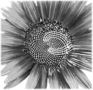
2. F12+F22+···+Fn2= FnFn+1.
3. If n ≥ 2, then (Fn)2−Fn+1Fn−1 = (−1)n+1.
= (Fn)2+2FnFn−1 +(Fn−1)2−Fn+1Fn −(Fn)2 = (Fn−1)2+Fn(2Fn−1 −Fn+1)
= (Fn−1)2+Fn(2Fn−1 −(Fn +Fn−1))
= (Fn−1)2+Fn(Fn−1 −Fn)
= (Fn−1)2−FnFn−2 = (−1)(n−1)+1= (−1)(n+1)+1,
Definition 6.4.7. Let A be a set. Let G(A) be the set defined by
| G(A) = | ∞ n=1� |
|
△ |
|---|
| Exercises |
|---|
Exercise 6.4.1. Let r1,r2,r3,... be the sequence defined by r1 = 1, and rn+1 = 4rn +
Exercise 6.4.4. [Used in Exercise 4.4.20.] Let A be a non-empty set, and let f : A → A be a function. Suppose that f is bijective. Prove that fnis bijective for each n ∈ N. Exercise 6.4.5. For each n ∈ N, find an example of a function f : A → A for some set A such that fnis a constant map, but fris not a constant map for all r ∈ {1,...,n−1}. Exercise 6.4.6. [Used in Proposition 6.4.6.] Prove Proposition 6.4.6 (1) (2).
Exercise 6.4.7. [Used in Section 8.6.] Let n ∈ N. Exercise 6.4.9. [Used in Section 8.6.] Let n,k ∈ N. Suppose that k ≥ 2. Prove that each of the following holds.
be a sequence satisfying An+2 = cAn+1 +dAn for all n ∈ N. (By Theorem 6.4.5 there is a unique such sequence for each choice of A1 and A2.) Let |
||
|---|---|---|
|
and | |
220 6 Finite Sets and Infinite Sets
(4) Apply Part (3) of this exercise to the Fibonacci sequence, and deduce Equa- tion 6.4.1.
13
(i) (ii)
| 6.5 Cardinality of Sets | 221 |
|---|---|
who is familiar, at least informally, with limits of sequences. (We will discuss limits of sequences rigorously, albeit briefly, in Section 7.8; see any introductory text in real looking at successive ratios of Fibonacci numbers, that is, the numbers 1, 2 1, 3 2, 5 3, 8 5, 13 8,··· . |
|
6.5 Cardinality of Sets
Intuitively, we know what it means to talk about the “size” of a finite set, and it seems intuitively clear that finite sets come in different sizes. What about infinite sets? Does it make sense to discuss the “size” of an infinite set, and if it does, do infinite sets come in different sizes? Galileo, writing in the early seventeenth century in [Gal74, pp. 38–47], thought that all infinite sets had the same size. Though he had some very good insights into infinite sets, even the brilliant Galileo was mistaken on this matter, as we shall see below. A correct understanding of the sizes of infinite sets was due to Cantor, the developer of set theory, two and a half centuries after Galileo. In the remaining sections of this chapter we will see a number of important arguments by Cantor; these ideas helped propel set theory into its prominent role in modern mathematics.
To determine whether two sets have the same size, we will try to pair up the elements of the two sets. Our tool for “pairing up” is bijective functions, as in the following definition.
Definition 6.5.1. Let A and B be sets. The sets A and B have the same cardinality, denoted A ∼ B, if there is a bijective function f : A → B. △ Observe that Definition 6.5.1 refers only to whether two sets have the “same cardinality”; nothing is stated about the “cardinality” (which means size) of each of the two sets. Using bijective functions allows us to compare two sets, but not to say anything about each of the individual sets.
3. If A ∼ B and B ∼ C, then A ∼ C.
Proof. See Exercise 6.5.3. ⊓⊔
Example 6.5.3.
(1) Though he made one major mistake concerning infinite sets (to be discussed shortly), Galileo understood the idea of using bijective functions (as we now call them) to show that two sets have the same cardinality. In the following quote from [Gal74, pp. 40–41], Galileo discusses some sets of positive natural numbers in a dialogue between two of his protagonists.
In modern terminology, Galileo states that the set of natural numbers N = {1,2,3,...} and the set of squares S = {1,4,9,16,...} have the same cardinality. Galileo’s argument is precisely the same as our modern one, which is that there is a bijective function h: N → S. The function h that Galileo suggests is the most natural follows from the fact that k: S → N defined by k(n) =√n for all n ∈ S is an inverse of h, where we make use of Theorem 4.4.5 (3). one to use, namely, the function defined by h(n) = n2for all n ∈ N. That h is bijective (2) The set of natural numbers N and the set of integers Z have the same cardi-nality. One choice of a bijective function f : N → Z is the one defined by (3) Let a,b,c,d ∈ R. Suppose that a
< b and c < d. We will show that [a,b]
∼[c,d], that (a,b) ∼ (c,d),
and similarly for half-open intervals. Let g: [a,b]
→ [c,d] be defined by |
|---|
1. A set is finite if it is either the empty set or it has the same cardinality as
2. A set is infinite if it is not finite. {1,...,n} for some n ∈ N.
Lemma 6.5.5.
1. The set N is infinite.
contradiction. Hence N is not finite, and so it is infinite. f({1,...,n}). Because f(k) + 1 ∈ N, we deduce that f is not surjective, which is a
further that B is finite. It would then follow from Exercise 6.5.5 that N is finite, which (2). Let B be a set. Suppose that B is countably infinite. Then B ∼ N. Suppose
In this quote Galileo essentially says that all infinite sets have the same cardi-nality, which would make them all countably infinite in our terminology. In fact, we will see in Corollary 6.5.8 below that Galileo was wrong, and that there are indeed uncountable sets. To prove that corollary, we make use of the cardinality of the power set of a set. We start with an example.
Example 6.5.6. Let A = {1,2}. Then P(A) = {/0,{1},{2},{1,2}}. Therefore A ̸∼P(A). ♦
Next, suppose that A ̸= /0. Suppose further that A ∼ P(A). Then there is a bijective function f : A → P(A). Let D = {a ∈ A | a /∈ f(a)}. Observe that D ⊆ A, and so D ∈ P(A). Because f is surjective, there is some d ∈ A such that f(d) = D. Is d ∈D? Suppose that d ∈ D. Then by the definition of D we see that d /∈ f(d) = D. Suppose that d /∈ D. Then d ∈ f(d) = D. We therefore have a contradiction, and so A ̸∼ P(A). ⊓⊔
In the following proof we will use Theorem 6.6.5 (1) from Section 6.6, though there is no circular reasoning here, because the proof of Theorem 6.6.5 does not make use of the corollary we are about to prove.
We conclude this section with two important theorems concerning cardinalities of sets. The proofs of these theorems are much trickier than what we have seen so far in this section. We start with the following definition.
Definition 6.5.9. Let A and B be sets. We say that A ≼ B if there is an injective function f : A → B; we say that A ≺ B if A ≼ B and A ̸∼ B. △ Intuitively, if A ≺ B, then A has “smaller size” than B. Some basic properties of the relation ≼ are given in Exercise 6.5.11. It is simple to see that for any set A, there is an injective function A → P(A), and hence A ≼ P(A); by Theorem 6.5.7 we see that A ≺ P(A). Applying this fact to the set N, and then to P(N), to P(P(N)) and so on, we deduce that
concept of ≼. Although our notation (which looks suspiciously like ≤) might make it appear as if these results are trivial, in fact neither is trivial at all.
Our first theorem, called the Schroeder–Bernstein Theorem (also known as the
The idea of the proof of the Schroeder–Bernstein Theorem, the bulk of which
is contained in the proof of the following lemma, is as follows. Let A, B and C be
However, although h is certainly surjective, and although the restriction of h to each
of A − B and B is injective, it is not the case that h as a whole is injective, because there is overlap between g(A−B) and B. We would then want to modify h by letting it equal the identity on only some subset of B, which would hopefully eliminate the
of writing the same thing.
Lemma 6.5.11. Let A, B and C be sets. Suppose that C ⊆ B ⊆ A, and that A ≼ C. Then A ∼ B.
g(T) = g� ∞n=0�Tn�=
n=0�g(Tn) =
Let h: A → B be defined by
h(x) =�g(x),
x,y ∈ A−T, then h(x) = h(y) implies x = y. If x ∈ T and y ∈ A−T, then h(x) = h(y) implies g(x) = y, which implies that y ∈ g(T) ⊆ T, which is a contradiction, and hence this case is not possible. The case where x ∈ A−T and y ∈ T is similarly not possible. We conclude that h is injective.
Let b ∈ B. First, suppose that b ∈ T. Because b /∈ A − B = T0, then b ∈ Tk for some k ∈ N. Hence b ∈ g(Tk−1), which means that b = g(z) for some z ∈ Tk−1 ⊆ T. Because z ∈ T, then b = h(z). Second, suppose that b ∈ B−T. Then b ∈ A−T, and hence h(b) = b. We conclude that h is surjective, and it follows that h is bijective. ⊓⊔
T0,T1,... and the function h in the proof of Lemma 6.5.11 for a simple example.
The benefit of using the Schroeder–Bernstein Theorem is that there are cases
entirely satisfying, because it would be nicer to see an explicit bijective function We mention that whereas the above proof that (a,b) ∼ [a,b] is short, it is not
f : [a,b] → (a,b). The reader is asked to find such a function in Exercise 6.5.14,
upon the Axiom of Choice. It is not just for convenience that we make use of this
axiom, but it is a necessity, because the Trichotomy Law for Sets is in fact equivalent
Theorem 6.5.13 (Trichotomy Law for Sets). Let A and B be sets. Then A ≼ B or
B ≼ A.
b = c. We conclude that�(c,e),(d,e) ∈�(c,e) and (d,e) must both be in some K ∈ C, and because K is an injective partial F∈CC, for some c,d ∈ A and e ∈ B. A similar argument shows that F∈CF is a partial function from A to B. Next, suppose that
function, then it must be the case that c = d. We conclude that�partial function from A to B, and hence that�By Zorn’s Lemma (Theorem 3.5.6) the family of sets P has a maximal element. F∈CF ∈ P. F∈CF is an injective
| 230 |
|---|
Exercise 6.5.1. Prove that the set of all integers that are multiples of 5 has the same
cardinality as the set of all integers.
Exercise 6.5.5. [Used repeatedly.] Let A and B be sets. Suppose that A ∼ B. Prove that if A is finite, infinite, countably infinite, countable or uncountable, then so is B.
Exercise 6.5.6. [Used in Theorem 6.7.4 and Exercise 6.7.1.]
finite, and that A is respectively finite, infinite, countably infinite, countable or un-
countable.
Exercise 6.5.10. Let A, B, C and D be sets. Suppose that A ∼ B and C ∼ D. Prove that A×C ∼ B×D.
Exercise 6.5.11. [Used in Section 6.5.] Let A, B and C be sets.
However, in order to see a concrete example of how the proof of Lemma 6.5.11 (and
hence of the Schroeder–Bernstein Theorem) works, the reader is asked to compute
(2) Let X,Y ⊆ R be subsets. If (a,b) ⊆ X and (c,d) ⊆ Y, then X ∼ Y.
Exercise 6.5.14. [Used in Example 6.5.12.] Let a,b ∈ R. Suppose that a < b. We saw in Example 6.5.12 that [a,b] ∼ (a,b). That proof was apparently brief, though the brevity was illusory, because the proof relied upon our work proving first Zorn’s Lemma (Theorem 3.5.6), and then the Schroeder–Bernstein Theorem (The-orem 6.5.10). Moreover, the proof in Example 6.5.12 did not explicitly exhibit a bijective function between the two intervals, and as such is not as concrete as possi-ble.
[f(A)− f(V)] = /0. P(A) such that g(V) = V. Prove that B = V ∪ [f(A) − f(V)], and that V ∩[Use Exercise 3.3.13 (1).] (2) Let h: A → B be defined by
h(x) =�x, f(x), if x ∈ A−V if x ∈ V.
232 6 Finite Sets and Infinite Sets
For sets in general, we did not assign a numerical value to each set that would be called the “size” of the set, because for infinite sets we would need to assign something other than real numbers (each of which is finite), and given what we have at our disposal in this text there are no other such “numbers” we can use. See [Pot04, Chapters 9 and 12] and [HJ99, Chapters 5 and 6] for discussion of cardinal and ordinal numbers, which are different types of “infinite numbers” that are relevant to the cardinality of sets.
Although Corollary 6.6.3 seems rather obvious, it actually tells us something of real substance. Recall the problem of finding hotel rooms for people mentioned at the start of this section. We stated that there were two ways to compare the size of the set of people wanting to stay at the hotel and the size of the set of available hotel rooms: pairing up elements of the two sets, or counting the number of elements in each set and comparing the numbers. In the two approaches we compare different things, namely, sets in the first approach and numbers in the second. Corollary 6.6.3 tells us that we will always obtain the same result by either method.
Example 6.6.4. Let B = {1,4,9,16}. We can formally show that |B| = 4 by showing that B ∼ {1,...,4} = {1,2,3,4}. To prove this last claim, let h: B → {1,...,4} be defined by h(x) =√x for all x ∈ B. It is easy to verify that the function h is bijective. Needless to say, the use of a formal proof to demonstrate that |B| = 4 in this particular case is a bit of overkill, and we will not feel the need to give any more such proofs concerning the cardinalities of such finite sets. It is nice to know, however, that such proofs can be constructed. ♦
Theorem 6.6.5. Let A be a set. Suppose that A is finite.
1. If X ⊆ A, then X is finite.
(2). If A−X = /0, then the result is trivial, so assume otherwise. Let n = |A|. Be-cause A−X ̸= /0, then A ̸= /0, and therefore n ̸= 0. Let f : A → {1,...,n} be a bijective function. We can then apply Theorem 6.3.11 (2) to the subset f(X) of {1,...,n} to find a bijective function g: {1,...,n} → {1,...,n} such that g(f(X)) = {1,...,k} for some k ∈ N such that k ≤ n. By Lemma 4.4.4 (3) we see that g ◦ f is bijective. It then follows from Exercise 6.5.4 and Exercise 4.3.5 that X ∼ {1,...,k}, which means that |X| = k. Using Exercise 4.3.5 again and Exercise 4.4.11, we see that
(g◦ f)(A−X) = (g◦ f)(A)−(g◦ f)(X) = g(f(A))−g(f(X))
The following result is a simple corollary to Theorem 6.6.5 (1); details are left to
the reader.
proper subset of Z, and yet we saw in Example 6.5.3 (2) that N ∼ Z. In fact, as we will see in Theorem 6.6.12 below, Theorem 6.6.5 (4) completely characterizes finite
sets. In order to prove this characterization, however, we need to learn more about
that the elements of N are lined up. As an example of how to line up the elements of a
countably infinite set, recall Example 6.5.3 (2), in which we saw a bijective function
For our first result about countable sets, recall that Theorem 6.6.5 (1) stated that a subset of a finite set is finite. The following theorem shows that the analogous result is true for countable sets as well. This theorem shows why it is often useful to work with the broader concept of countable sets, rather than the narrower concept of countably infinite sets, because the theorem would not be true if we replaced“countable” with “countably infinite”; observe that a subset of a countably infinite set need not be countably infinite, because it can be finite.
The intuitive idea of the proof of the theorem is as follows. The interesting case in the proof is when X is an infinite subset of N. Because X is non-empty, we can apply the Well-Ordering Principle (Theorem 6.2.5) to find some c1 ∈ X such that c1 ≤ x for all x ∈ X. Then c1 < x for all x ∈ X −{c1}. Let X2 = X −{c1}. Because X is infinite, then X2 ̸= /0, and by the same argument as before there is some c2 ∈ X2 such that c2 < x for all x ∈ X2 −{c2} = X −{c1,c2}. Let X3 = X −{c1,c2}. We can continue this process forever, and we therefore obtain a sequence c1,c2,c3,... in X such that c1 < c2 < c3 < ···. The rest of the proof consists of showing that this sequence in fact contains all the elements of X. Because all the elements of X can be lined up c1,c2,c3,..., and because X is infinite, it follows that X is countably infinite. How-ever, the phrase “we can continue this process forever” is not rigorous, and we make this proof rigorous by using the version of Definition by Recursion given in Theo-Before proceeding, the reader should review the notation given in Definition 6.4.7. rem 6.4.8. The function f : N → A in the proof replaces the sequence c1,c2,c3,....
By the Well-Ordering Principle (Theorem 6.2.5), there is a unique element b ∈X such that b ≤ x for all x ∈ X. Let k: G(X) → X be defined as follows. Let g ∈G(X). Then g ∈ F ({1,...,n},X) for some n ∈ N, which means that g is a function {1,...,n} → X. It follows from Exercise 6.6.3 that g cannot be surjective, and hence X −g({1,...,n}) ̸= /0. Using the Well-Ordering Principle again we see that there is a unique element zg ∈ X −g({1,...,n}) such that zg ≤ x for all x ∈ X −g({1,...,n}). We then let k(g) = zg.
We can apply Theorem 6.4.8 to b and k as above, and we deduce that there is
⊓⊔
In order to show that a set is countable, it is necessary to show that it is either
Theorem 6.6.8. Let A be a non-empty set. The following are equivalent.
a. The set A is countable.
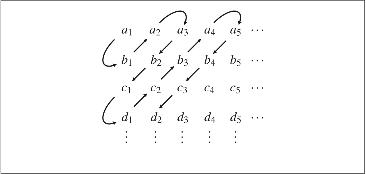
236 6 Finite Sets and Infinite Sets
The best we can do regarding unions and products of countable sets is seen in the following two theorems. To form an intuitive picture of why the union of countably many countable sets is itself countable, consider first the union of two countable sets A and B. We can line up each of their elements as a1,a2,... and b1,b2,.... We can then line up the elements of A ∪ B as a1,b1,a2,b2,..., where we drop any element that is the same as an element previously listed (which could happen because A and B might have elements in common). A picture for the union of countably many countable sets is seen in Figure 6.6.1, where the elements of the union are “lined up”in the order shown by the arrows, and where again we drop any element that is the same as an element previously listed.
Fig. 6.6.1.
| 6.6 Finite Sets and Countable Sets | 237 |
|---|---|
and therefore that Ai ̸= /0 for all i ∈ I. There are two cases, depending upon whether I is countably infinite or is finite. We prove the former case, leaving the other case to the reader in Exercise 6.6.12.
some w ∈ N such that x = fk(w).
Let t = k +w − 1. The reader can then verify
that g((t set of all surjective functions N → Ai for each i ∈ I, and we would apply the Ax-iom of Choice to the family of sets {Si}i∈I; we omit the details. It is pointed out in [Vau95, p. 56] that any proof of Theorem 6.6.9 (2) requires the Axiom of Choice. Theorem 6.6.10. Let A1,...,An be sets for some n ∈ N. Suppose that A1,...,An are countable. Then A1 ×···×An is countable. |
|
| to the reader. | ⊓⊔ |
intuitively plausible that countably infinite sets are the “smallest.” We now have the tools to prove this fact.
Theorem 6.6.11. Let A be a set. If A is infinite, then A has a countably infinite subset.
Theorem 6.6.12. Let A be a set. Then A is finite if and only if A has no proper subset with the same cardinality as A.
Proof. Suppose that A is finite. Let X ⫋ A. Theorem 6.6.5 (4) implies that X ̸∼ A. Suppose that A is infinite. Then by Theorem 6.6.11 we know that A has a count-ably infinite subset. Let X ⊆ A be countably infinite. By Exercise 6.6.6 there is a function f : X → X that is injective but not surjective. Let g: A → A be defined by
reader is asked to prove this fact in Exercise 6.6.4. For an infinite set B, by contrast, f : A → A is bijective if and only if it is injective if and only if it is surjective. The
a surjective or injective function g: B → B need not be bijective; an example of an injective function that is not surjective is used in the proof of Theorem 6.6.12, and any left inverse of such a function would be surjective but not injective.
| Exercises |
|---|
Exercise 6.6.5. [Used in Section 8.2.] Let F ⊆ N be a set. Suppose that F is finite and non-empty. Use Theorem 6.3.11 (1) to prove that there is some k ∈ F such that p ≤ k for all p ∈ F.
Exercise 6.6.6. [Used in Theorem 6.6.12.] Let X be a set. Suppose that X is countably
are countable. Prove that A×B is countable.
Exercise 6.6.9. Let A and F be sets. Suppose that A is countably infinite set, and that
Exercise 6.6.10. Let A be an uncountable set, and let T be any non-empty set. Prove
that A×T is uncountable.
S = {b ∈ B | k−1({b}) has more than one element}.
Prove that if S is infinite, or if k−1({t}) is infinite for some t ∈ S, then k has infinitely many right inverses.
the cardinality of the standard number systems, which are the natural numbers, the
integers, the rational numbers, the real numbers and the complex numbers. Of course,
of this book; see [Blo11, Theorem 2.6.13] for details. It therefore might appear that
there are “more” rational numbers than integers. The following theorem shows that
positive rational numbers: follow the path indicated by the arrows, and drop every
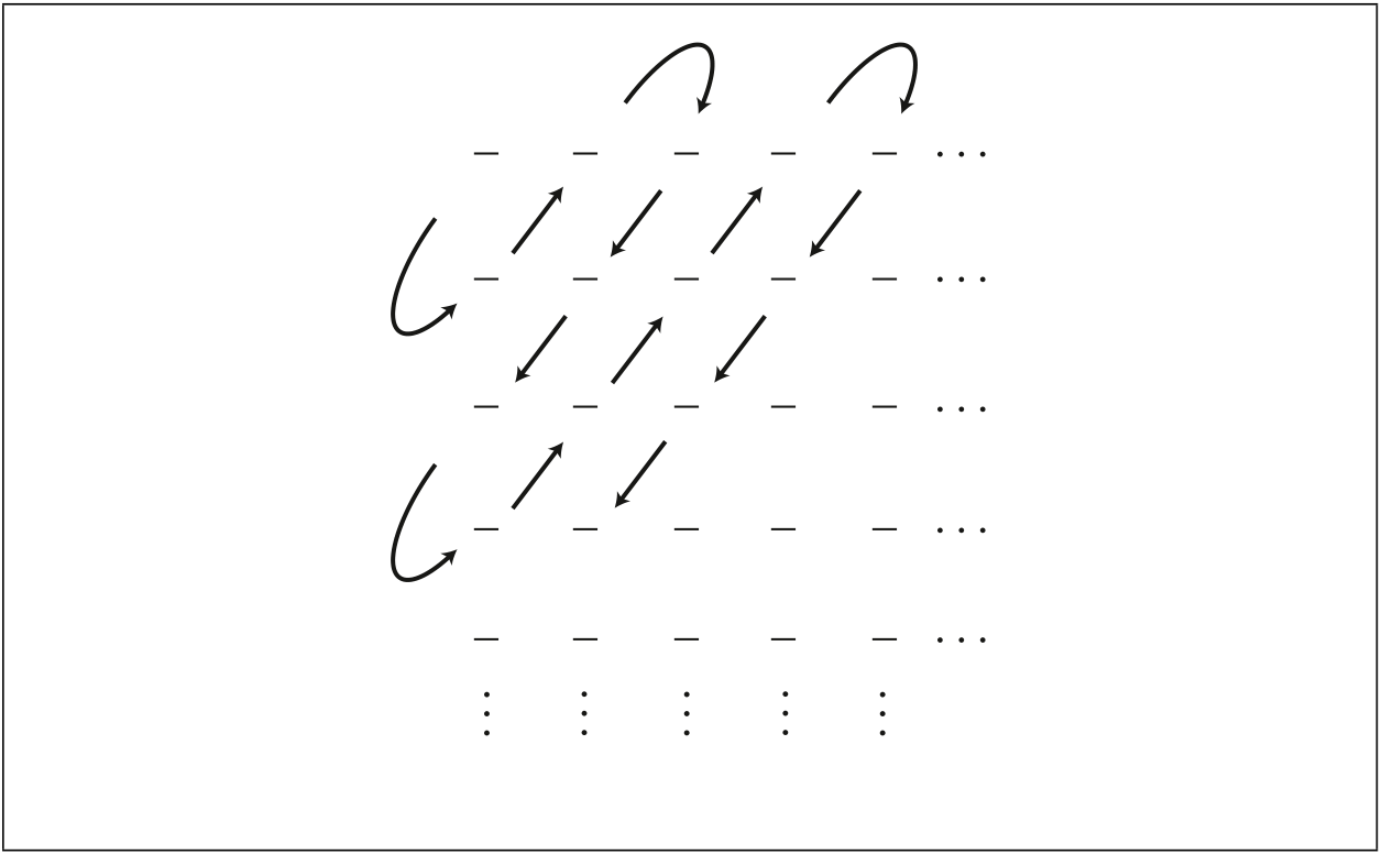
| 1 | 1 | 1 | 1 | |
|---|---|---|---|---|
| 1 | 2 | 3 | 4 | |
| 2 | 2 | 2 | 2 |
|
| 1 | 2 | 3 | 4 |
|
| 3 | 3 | 3 | 3 | |
| 1 | 2 | 3 | 4 | |
| 4 | 4 | 4 | 4 | |
| 1 | 2 | 3 | 4 | |
| 5 | 5 | 5 | 5 |
|
| 1 | 2 | 3 | 4 |
|
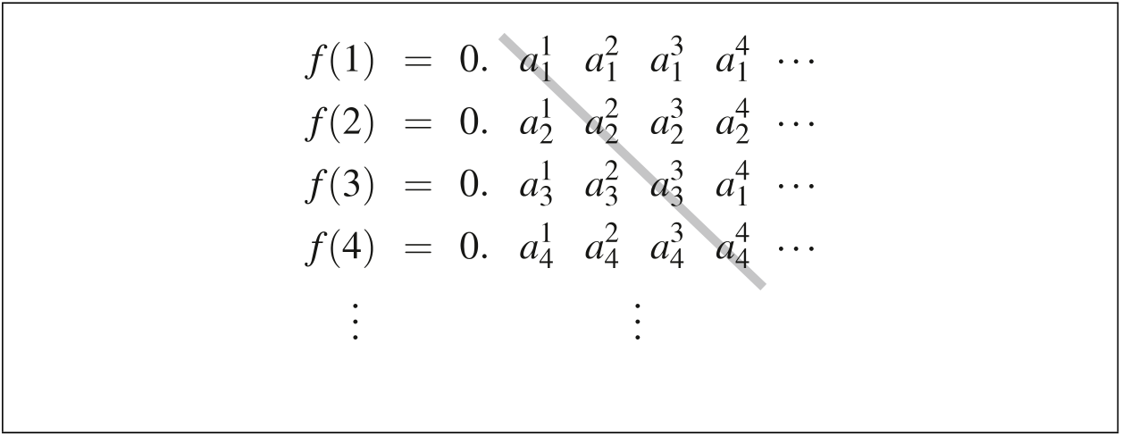
242 6 Finite Sets and Infinite Sets
be a bijective function. For each n ∈ N, we can write f(n) as an infinite decimal
and where the expansion does not eventually become the number 9 repeating. f(n) = 0.a1 na2 na3 n..., where the numbers a1 n,a2 n,a3 n,... are integers in {0,1,...,9},
k= 1.
Observe that bk ̸= ak kfor all k ∈ N. Let b be the number represented by the decimal
each n ∈ N, the n-th digit in the decimal expansion of f(n) is an n, whereas the n-th
digit in the decimal expansion of b is bn. Hence b ̸= f(n) for all n ∈ N. We have therefore reached a contradiction to the surjectivity of f, and we deduce that R is not
Fig. 6.7.2.
Although Cantor’s diagonal argument is a very nice proof, it is not quite as sim-
cult than might be expected, in part because it relies upon the Least Upper Bound
244 6 Finite Sets and Infinite Sets
inclusion function i: N → R is injective. From Theorem 6.7.3 we know that N ≺ R. Is there a set X such that N ≺ X ≺ R? Cantor conjectured that there was no such set, and this conjecture is known as the Continuum Hypothesis. You might be tempted to try to look for such a set yourself, but you will not succeed. Nor, amazingly enough, will you succeed in proving that no such set exists. Due to the remarkable work of Kurt G¨odel in 1938 and Paul Cohen in 1963, it turns out that the Continuum Hypoth-esis is independent of the Zermelo–Fraenkel Axioms for set theory (see Section 3.5 for a discussion of these axioms). In other words, the Continuum Hypothesis can nei-ther be proved nor disproved from the Zermelo–Fraenkel Axioms. See [Mal79, Sec-tion 1.12] or [Vau95, Section 7.7] for further discussion (though the proof of Cohen’s result is to be found only in more advanced texts). It follows that we either need to be satisfied with not being able to resolve the Continuum Hypothesis, or we need to find new axioms for set theory. Mathematicians have stuck to the standard axioms, because they have worked well so far, and therefore have decided to live with the odd situation regarding the Continuum Hypothesis.
binom n 0 = 1
binom n k = if k == n then 1
example, the allowed symbols include the letters of the English alphabet (uppercase and lowercase versions of the same letter are considered to be different symbols), the digits 0,...,9, various symbols such as =, :, [, ] and so on, and a blank space (which we also think of as a symbol). Repeated blank spaces and new lines are ignored by the computer (though they make it easier for human beings to read the code), so we can ignore them too. For a given computer programming language, let Σ denote the set of all possible symbols used, including the blank space symbol. The set Σ is always finite. Using the symbols in Σ, we can then write computer programs, which are simply certain finite strings of symbols in Σ, though of course not all strings will be valid programs. Let S(Σ) denote the set of all finite strings with symbols in Σ, and let C(Σ) denote the set of all valid programs using symbols in Σ. Then C(Σ) ⊆ S(Σ). As stated above, a computer program causes the computer to take various input data, and for each possible input, produce some output data. For a computer pro-gram written with the symbols Σ, both the input and the output are finite strings of symbols in Σ. Therefore each computer program in Σ causes the computer to F (S(Σ),S(Σ)), using the notation of Section 4.5. Putting these observations together, act as a function S(Σ) → S(Σ). The collection of all such functions is denoted we see that each programming language using symbols in Σ gives rise to a function Φ : C(Σ) → F (S(Σ),S(Σ)), where for each computer program p written with sym-bols in Σ, we obtain the function Φ(p): S(Σ) → S(Σ). Our question stated above asking whether there is a computer programming lan-guage with which we could make the computer do anything we might wish it to do can now be expressed by asking whether there is some programming language such that the corresponding function Φ is surjective. If Φ were surjective, then every pos-sible function S(Σ) → S(Σ) could be obtained from at least one computer program. On the other hand, if Φ were not surjective, then there would be at least one function S(Σ) → S(Σ) that we might want the programming language to do that could not be achieved.
The answer to our question is that regardless of the programming language and the set of symbols Σ used, and regardless of the computer used, the function Φ is never surjective. The reason is that C(Σ) is always countable, and F (S(Σ),S(Σ)) is always uncountable. The fact that there cannot be a surjective function from a countable set to an uncountable one follows from Theorem 6.6.8; the details are left to the reader.
| 246 | ||
|---|---|---|
| We therefore see that cardinality considerations imply that there is a theoretical limitation to what can be accomplished by computer programming. See [Har96] for | ||
| further discussion. | ♦ | |
Exercise 6.7.1. Which of the following sets is countable, and which has the same cardinality as R? Informal justification is acceptable.
|
|---|
S = {x ∈ (0,1) | the decimal expansion of x has only odd digits}
is uncountable.
Exercise 6.7.4. [Used in Theorem 6.7.5.]
(1) Prove that (0,1)×(0,1) ∼ (0,1). Use the fact that every real number can be expressed uniquely as an infinite decimal, if decimal expansions that eventu-
cardinality as R.
Exercise 6.7.6. Let D be a partition of R such that each element of D is an interval
Exercise 6.7.8. [Used in Section 6.7.] The purpose of this exercise is to prove that
P(N) ∼ R. As in the proof of Theorem 6.7.3, it will suffice to prove that P(N) ∼(0,1). We will use the facts about decimal expansions of real numbers that were
expansions.
By the Schroeder–Bernstein Theorem (Theorem 6.5.10), it will suffice to prove
Exercise 6.7.9. [Used in Section 6.7.] In Theorem 6.7.1 we saw that the set Q is
countably infinite, which told us that in principle the elements of Q could be “lined
numbers were lined up by following the arrows, and dropping every fraction that
is equal to one that had already been encountered. In this exercise we discuss an
The alternative way of lining up the positive rational numbers is represented by
the following diagram.
................................................................. ................................................................. ............ ................................................................. ................................................................. ............
1 3 2 3
... ... ... ...
This diagram is constructed using Definition by Recursion, starting with1 1, and
as a fraction in lowest terms, is obtained precisely once by this procedure. We can
therefore line up the positive rational numbers by stringing together the successive
and only if the two numbers a and b are relatively prime, as defined in Exercise 2.4.3.
As in Exercise 4.4.8, let L be the set defined by
An = {c1 n,c2 n,...,c2n−1 }.
We define these elements using Definition by Recursion as follows. Let c1 1= (1,1).
may also be other elements of L in Sn, but that does not matter.)
(2) All the elements in Sn are distinct, which means that cx i= cy jif and only if
Having completed the basics, we now turn to a number of additional top-ics. These topics were chosen because they contain accessible ideas from important areas of modern mathematics, and because they make use of the concepts we have learned so far. Due to space limitations, we will be a bit more terse in this part of the text than previously. Each section of Chapter 7 gives a very brief introduction to a particular topic; further details await courses in those areas. Section 7.1 treats binary operations, Sections 7.2 and 7.3 treat groups, Sections 7.4 and 7.5 treat partially or-dered sets and lattices, Sections 7.6 and 7.7 treat enumeration, and Sec-tion 7.8 treats limits of sequences. In Chapter 8 we let the reader take over. In each of Sections 8.2–8.7 we briefly introduce a topic, which the reader is then urged to explore on her own; in Section 8.8 the reader has the opportunity to assume the role of a mathematics professor and critique some attempted proofs taken from actual homework exercises submitted by students.
7
Among the most basic topics taught in elementary school mathematics are opera-tions such as addition and multiplication of numbers. Each such operation takes two numbers, and produces a single resulting number. Another type of operation is nega-tion of numbers, which takes a single number and produces another number. We can formalize both these types of operations using sets and functions.
Definition 7.1.1. Let A be a set. A binary operation on A is a function A×A → A. A unary operation on A is a function A → A. △ Let A be a set, and let ∗: A×A → A be a binary operation. If a,b ∈ A, then it would be proper to denote the result of doing the operation ∗ to the pair (a,b) by writing ∗((a,b)). Such notation is quite cumbersome, however, and would not look like familiar binary operations such as addition of numbers. Hence, we will write Binary operations are used throughout mathematics. We will prove only one very a∗b instead of ∗((a,b)).
Undergraduate Texts in Mathematics, DOI 10.1007/978-1-4419-7127-2_7,
© Springer Science+Business Media, LLC 2011
| ⋆ | p q r |
|---|---|
| p r p qq p q r r r p |
(1) The binary operations addition and multiplication on Z are both commutative. The binary operation subtraction on Z is not commutative; for example, we see that 5−2 ̸= 2−5.
(2) The binary operation · defined in Example 7.1.2 (2) is not commutative. The reader should supply an example of two matrices A,B ∈ GL2(R) such that A · B ̸= B · A. Some pairs of matrices in GL2(R) can be multiplied in either order without changing the result, for example is not the case that all pairs can be multiplied in either order without changing the�3 0�·� 5 0�=� 5 0�·� 3 0�; however, because it
(1) The binary operations addition and multiplication on Z are both associative. The binary operation subtraction on Z is not associative; for example, we see that (5−2)−1 ̸= 5−(2−1).
can be proved directly by a tedious computation, or indirectly by using more ad-(2) The binary operation · defined in Example 7.1.2 (2) is associative. This fact
254 7 Selected Topics
Definition 7.1.7. Let A be a set, and let ∗ be a binary operation on A. An element e ∈ A is an identity element for ∗ if a∗e = a = e∗a for all a ∈ A. If ∗ has an identity element, the binary operation ∗ satisfies the Identity Law. △
not have an identity element. Even though n − 0 = n for all n ∈ N, we observe that 0−n ̸= n when n ̸= 0. namely, the identity matrix to the column below ⋆, and the row to the right of q is identical to the row to the right of ⋆. |
|---|
matically.
Lemma 7.1.9. Let A be a set, and let ∗ be a binary operation on A. If ∗ has an identity element, the identity element is unique.
| ∗ | e a b c d |
|---|---|
| e e a b c da a b e d eb b e c e ac c d e a c d b a c b |
| Exercises |
|---|
Exercise 7.1.1. Which of the following formulas defines a binary operation on the
given set?
(4) Let ◦ be defined by (x,y)◦ (z,w) = (x + z,y +w) for all (x,y),(z,w) ∈ R2− {(0,0)}.
(5) Let ⊙ be defined by x⊙y = |x+y| for all x,y ∈ N.
(1) The binary operation ⊕ on Z defined by x⊕y = −xy for all x,y ∈ Z.
(2) The binary operation ⋆ on R defined by x⋆y = x+2y for all x,y ∈ R. (3) The binary operation ⊗ on R defined by x⊗y = x+y−7 for all x,y ∈ R.
element and, if there is an identity element, which elements have inverses. (Do not
check for associativity.)
| (1) | (4) |
|
|||||
|---|---|---|---|---|---|---|---|
| (2) | (5) | ||||||
|
|||||||
| (3) |
Exercise 7.1.4. [Used in Section 7.2.] Find an example of a set and a binary opera-
7.2 Groups 257
Exercise 7.1.5. Let n ∈ N. Recall the definition of the set Zn and the binary operation· on Zn given in Section 5.2. Observe that [1] is the identity element for Zn with respect to multiplication. Let a ∈ Z. Prove that the following are equivalent. a. The element [a] ∈ Zn has an inverse with respect to multiplication.
7.2 Groups
As discussed in Section 7.1, some binary operations satisfy various nice properties, such as associativity and commutativity, whereas others do not. Certain combinations of these properties have been found, in retrospect, to be particularly widespread and useful. The most important such combination of properties is given in the following definition.
Among many other uses, Definition 7.2.2 gives rise to the following
well-known mathematical joke. Question: What is purple and commutative?
Answer: An abelian grape. (Mathematical jokes are rather scarce, so one
cannot be overly picky about their quality.)
Groups are relatively recent by mathematical standards, having arisen in
the nine-teenth century, but they are now important in a wide variety of
areas of both pure and applied mathematics, including geometry,
algebraic topology, quantum mechanics and crystallography, to name just
a few. Crystallography makes use of the centrality of groups in the
rigorous study of symmetry. See [Fra03] or [Rot73], among many possible
texts, for a more detailed treatment of group theory; see [Arm88] or
[Bur85] for the connection between group theory and symmetry; and see
[LP98, Chapter 6] for some applications of group theory. Our brief
discussion of groups, in this section and the next, cannot even begin to
hint at the many fascinating aspects of this topic.
The term “group” is one of those words that has a standard colloquial meaning, and to which mathematicians have given a technical meaning that has little to do with the colloquial usage. The term “abelian” is in honor of the mathematician Niels Abel (1802–1829), who did important work in algebra.
| ◦ | e a b c |
|---|---|
| e a b c |
e e a b c a a b c eb b c e a c e a b |
omit the details, though the ambitious reader is invited to check all 64 cases. It is easy to verify that e is the identity element, by observing in the operation table for ◦ that the column below e is identical to the column below ◦, and similarly for the row to the right of e. The elements e and b are their own inverses, and a and c are inverses of each other. Hence (V,◦) is a group. It is easy to verify that ◦ is commutative, because the operation table is symmetric along the downward sloping diagonal. Hence (V,◦) is an abelian group.
(5) The pair (Z,⋆) given in Example 7.1.2 (3) is not a group. Although ⋆ does have an identity element, which is q, this binary operation is not associative, as dis-cussed in Example 7.1.6 (3), and the element p does not have an inverse. ♦
proof of Theorem 7.2.5 (4). a,b ∈ G are such that a∗b = e and b∗a = e, then b = a′. We will use this idea in the
The following theorem generalizes some familiar properties of (R,+), for exam-ple that −(x+y) = (−x)+(−y) for all x,y ∈ R.
(a∗b)∗(b′∗a′) = [(a∗b)∗b′]∗a′= [a∗(b∗b′)]∗a′
260 7 Selected Topics
the equation (a ∗ b)′= b′∗ a′. For an arbitrary group (G,∗), which does not neces-sarily satisfy the Commutative Law, it is not always true that (a∗b)′= a′∗b′for all a,b ∈ G. The reader is asked to provide such an example in Exercise 7.2.7. However, in the special case where (G,∗) is (R,+), and where a′is given by −a for all a ∈ R, then Theorem 7.2.5 (4) does indeed say exactly that −(x+y) = (−x)+(−y) for all x,y ∈ R. The fact that arbitrary groups do not necessarily satisfy the Commutative Law is also the reason why both Parts (1) and (2) of Theorem 7.2.5 are needed.
A useful consequence of Theorem 7.2.5 (1) (2) is that if the binary operation of a
because the leftmost column does not have the element n. On the other hand, just
because an operation table does have each element once and only once in each row
notion as follows.
Definition 7.2.6. Let (G,∗) be a group, and let H ⊆ G be a subset. The subset H is a subgroup of G if the following two conditions hold.
“closure” under the binary operation ∗ and the unary operation′.
Theorem 7.2.7. Let (G,∗) be a group, and let H ⊆ G be a non-empty subset. Then H is a subgroup of G if and only if the following two conditions hold.
an identity element, say ˆe. (We cannot assume, until we prove it, that ˆe is the same as e.) Then ˆe∗ ˆe = ˆe thinking of ˆe as being in H, and e∗ ˆe = ˆe thinking of ˆe as being in G. Hence ˆe∗ ˆe = e∗ ˆe. Because both ˆe and e are in G, we can use Theorem 7.2.5 (1) to deduce that ˆe = e.
Now let a ∈ H. Because (G,∗) is a group, the element a has an inverse a′∈ G. We will show that a′∈ H. Because (H,∗) is a group, then a has an inverse ˆa ∈ H. (Again, we cannot assume, until we prove it, that ˆa is the same as a′.) Using the definition of inverses, and what we saw in the previous paragraph, we know that a′∗a = e and ˆa∗a = e. Hence ˆa∗a = a′∗a. Using Theorem 7.2.5 (1) again, we deduce that a′= ˆa. Because ˆa ∈ H, it follows that a′∈ H. Therefore Property (ii) of the theorem holds. Now suppose that Properties (i) and (ii) hold. To show that H is a subgroup, we need to show that (H,∗) is a group. We know that ∗ is associative with respect to all the elements of G, so it certainly is associative with respect to the elements of H. Let b ∈ H. By Property (ii) we know that b′∈ H. By Property (i) we deduce that b′∗b ∈ H, and hence e ∈ H. Because e is the identity element for all the elements of G, it is certainly the identity element for all the elements of H. By Property (ii) we now know that every element of H has an inverse in H. Hence H is a group. ⊓⊔
(2) Let (G,∗) be a group. Let e be the identity element of G. Then {e} and G are both subgroups of G. The subgroup {e} is often called the trivial subgroup of G.
that the only subgroups of V are {e}, {e,b} and V. (3) Let (V,◦) be as in Example 7.2.3 (4). By checking all possibilities, it is seen♦
certain angles about the center of the triangle. In Figure 7.2.1 (ii) we see the three possible lines in which the plane can be reflected without changing the appearance of the triangle. Let M1, M2 and M3 denote the reflections of the planes in these lines. For example, if we apply reflection M2 to the plane, we see that the vertex labeled C is unmoved, and that the vertices labeled A and B are interchanged, as seen in Figure 7.2.1 (iii). The only two possible rotations of the plane about the center of the triangle that leave the appearance of the triangle unchanged are rotation by 120◦clockwise and rotation by 240◦clockwise, denoted R120 and R240. We do not need ro-tation by 120◦counterclockwise and rotation by 240◦counterclockwise, even though they also leave the appearance of the triangle unchanged, because they have the same net effect as rotation by 240◦clockwise and rotation by 120◦clockwise, respectively, and it is only the net effect of isometries that is relevant to the study of symmetry. Let I denote the isometry of the plane that does not move anything, that is, rotation by 0◦.
3
| 7.2 Groups | 263 |
|---|---|
this binary operation on G is associative. Observe that I is an identity element. It is |
|
(1) The set (0,1], and the binary operation multiplication.
(2) The set of positive rational numbers, and the binary operation multiplication. (3) The set of even integers, and the binary operation addition.
(7) The set Z, and the binary operation ⋄ on Z defined by a⋄b = a+b+1 for all a,b ∈ Z.
(8) The set R − {−1}, and the binary operation ⊙ on R − {−1} defined by a ⊙ b = a+b+ab for all a,b ∈ R−{−1}.
and only once in each row of the operation table and once and only once in each
column, but the set together with this binary operation is not a group.
Exercise 7.2.7. [Used in Section 7.2.] Find an example of a group (G,∗), and ele-ments a,b ∈ G, such that (a∗b)′̸= a′∗b′.
Exercise 7.2.8. Let A be a non-empty set, and let ∗ be a binary operation on A. Suppose that ∗ satisfies the Associative Law and the Identity Law, and that it also satisfies the Right Inverses Law, which states that for each a ∈ A there is an element b ∈ A such that a∗b = e, where e is the identity element for ∗.
b. aba′b′= e for all a,b ∈ G.
c. (ab)2= a2b2for all a,b ∈ G.
Exercise 7.2.10. Let (G,∗) be a group. Suppose that K ⊆ H ⊆ G. Prove that if K is a subgroup of H, and H is a subgroup of G, then K is a subgroup of G.
group.
(2) Suppose that n is not a prime number. Then n = ab for some a,b ∈ N such that 1 < a < n and 1 < b < n. Prove that the set {[0],[a],[2a],...,[(b−1)a]} is a subgroup of Zn.
tion of the symmetry group of an equilateral triangle in Example 7.2.10. Find all the
subgroups of the symmetry group of the square.
making it precise in the following definition.
Definition 7.3.1. Let (G,∗) and (H,⋄) be groups, and let f : G → H be a function. The function f is a homomorphism (sometimes called a group homomorphism) if
means that g is not a homomorphism.
(2) It is straightforward to verify that ((0,∞),·) is a group. Let h: R → (0,∞) be defined by h(x) = exfor all x ∈ R. Then h is a homomorphism from (R,+) to ((0,∞),·), because h(x+y) = ex+y= ex·ey= h(x)·h(y) for all x,y ∈ R.
first property states that γ is group homomorphism. It turns out that Z and Zn both
have the structure of a “ring,” which involves two binary operations (in this case
Homomorphisms of groups preserve the basic group structure, that is, the group
operation. The following theorem shows that a group homomorphism also preserves
3. If A ⊆ G is a subgroup of G, then f(A) is a subgroup of H. 4. If B ⊆ H is a subgroup of H, then f−1(B) is a subgroup of G.
Proof. We will prove Parts (2) and (3), leaving the rest to the reader in Exercise 7.3.6.
(3). By Corollary 7.2.8 we know that eG ∈ A, and by Part (1) of this theorem we know that eH = f(eG) ∈ f(A). Hence f(A) is non-empty. We can therefore use Theorem 7.2.7 to show that f(A) is a subgroup of H. Let x,y ∈ f(A). Then there are a,b ∈ A such that x = f(a) and y = f(b). Hence x⋄y = f(a)⋄ f(b) = f(a∗b), because f is a homomorphism. Because A is a subgroup of G we know that a ∗ b ∈ A, and hence x ⋄ y ∈ f(A). Using Part (2) of this theorem, we see that x′= [f(a)]′= f(a′). Because A is a subgroup of G, it follows from Theorem 7.2.7 (ii) that a′∈ A. We now use Theorem 7.2.7 to deduce that f(A) is a subgroup of H.⊓⊔
The most important method of combining functions is by composition. The fol-
given homomorphism is injective. We start with the following definition.
7.3 Homomorphisms and Isomorphisms 267
Example 7.3.6.
(1) Let g be as in Example 7.3.2 (2). The identity element of the group ((0,∞),·) is 1. Then kerg = g−1({1}) = {0}. Observe that the function g is injective.
injectivity of homomorphisms and triviality of kernels always holds.
Theorem 7.3.7. Let G and H be groups, and let f : G → H be a homomorphism. Let eG be the identity element of G. The function f is injective if and only if ker f = {eG}.
It follows that b ∗ a′∈ f−1({eH}) = ker f. Because ker f = {eG}, we deduce that b∗a′= eG. A similar calculation shows that a′∗b = eG. By Lemma 7.2.4 we deduce that (a′)′= b, and therefore by Theorem 7.2.5 (3) we see that b = a. Hence f is
injective. ⊓⊔
same.”
Definition 7.3.8. Let G and H be groups.
Example 7.3.9.
Let ({e},∗) and ({u},◦) be trivial groups. Let g: {e} → {u} be defined by g(e) = u. Then g(e∗e) = g(e) = u = u◦u = g(e)◦g(e). Hence g is a homomorphism. Clearly g is bijective, and hence it is an isomorphism.
|
|---|
| It can be verified that (Q,⋄) is a group; we omit the details. The group (V,◦) in Example 7.2.3 (4) also has four elements, but it is shown in Exercise 7.3.9 that (Q,⋄) and (V,◦) are not isomorphic. Intuitively, these groups are different in that all four elements of Q are their own inverses, whereas in V only two elements (the elements | |
|---|---|
| e and b) are their own inverses. | ♦ |
In Example 7.3.9 (3) we saw that there are at least two non-isomorphic groups with four elements. As seen in Exercise 7.3.10, it turns out that every group with four elements is isomorphic to one of these two groups. In general, it is quite difficult to take a natural number, and to describe all possible non-isomorphic groups with that number of elements, or even to say how many such groups there are; simply checking all possible operation tables (as is done in Exercise 7.3.10) is neither feasible nor satisfying with more than a few elements. The results are known for sufficiently small groups (up to 100 elements, for example), but there is no formula for the number of non-isomorphic groups with n elements for arbitrary n. See [Dea66, Section 9.3] or [Rot96, p. 85] for details.
tion has an inverse by Theorem 4.4.5 (3); hence f−1is defined without any regard to
the fact that f is a homomorphism.
| Exercises |
|---|
the homomorphisms are isomorphisms? The groups under consideration are (R,+),
and (Q,+), and ((0,∞),·).
Exercise 7.3.3. In this exercise we use the fact that (Zn,+) is a group for all n ∈ N, as was proved in Exercise 7.2.12 (1).
(1) Let j: Z4 → Z3 be defined by j([x]) = [x] for all [x] ∈ Z4, where the two appearances of “[x]” in the definition of j refer to elements in different groups.
(3) Can you find criteria on n,m ∈ N that will determine when the function r: Zn → Zm defined by r([x]) = [x] for all [x] ∈ Zn is well-defined and is a homomorphism? Prove your claim. Find the kernels for those functions that
are well-defined and are homomorphisms.
(2) (R − {0},·) and (R − {−1},∗), where x ∗ y = x + y + xy for all x,y ∈ R − {−1}.
(3) (R4,+) and (M2×2(R),+), where M2×2(R) is the set of all 2 × 2 matrices with real entries.
Exercise 7.3.10. [Used in Section 7.3.] Prove that up to isomorphism, the only two groups with four elements are (V,◦) of Example 7.2.3 (4) and (Q,⋄) of Exam-ple 7.3.9 (3). Consider all possible operation tables for the binary operation of a group with four elements; use the fact that each element of a group appears once in each row and once in each column of the operation table for the binary operation of the group, as remarked after Theorem 7.2.5.
7.4 Partially Ordered Sets
ties that a relation might satisfy, which are reflexivity, symmetry and transitivity. We
now turn our attention to a particular type of relation, which generalizes the order
our most general definition. These ideas are all made precise as follows.
Definition 7.4.1. Let A be a non-empty set, and let ≼ be a relation on A.
3. The relation ≼ is a total ordering (also called a total order or linear order-
ing) if it is a partial ordering, and if for every a,b ∈ A, at least one of a ≼ b or b ≼ a holds. If ≼ is a total ordering, the pair (A,≼) is a totally ordered
be looking at posets, rather than totally ordered sets, because the former are more
prevalent orderings. Observe that posets and totally ordered sets are all assumed to
(2) There are many relations that are reflexive and transitive but not antisymmet-
ric. For instance, any equivalence relation that has non-equal elements that are related
The relation < on these sets is not a partial ordering, because it is not reflexive. (3) Each of the sets N, Z, Q and R with the relation ≤ is a totally ordered set.
mentioned previously. (4) Let A be a set. Then (P(A),⊆) is a poset but not a totally ordered set, as
condition is dropped when w1 = w2). For example, we see that mandrel ≼ mandrill.
This relation, which is seen to be a total ordering, is called the lexicographical order
We form the Hasse diagram of a finite poset as follows. First, put a dot on the
page for each element of the poset, placed in such a way that if x ≼ y then y is higher
The Hasse diagram for this poset is given in Figure 7.4.1 (i). Observe that there is
no line segment from 2 to 8, even though 2 ≼ 8, because 8 does not cover 2. Also,
inition of “inequivalent” needs the notion of order preserving functions defined later
in this section, but we will use the term informally here. The Hasse diagrams of all
| (i) | (ii) | (iii) | (iv) | (v) |
|---|
We now turn to a definition that is slightly weaker than Definition 7.4.5. The following definition generalizes Definition 3.5.4 (1).
Definition 7.4.7. Let (A,≼) be a poset, and let a ∈ A. The element a is a maximal element of A if there is no x ∈ A such that a ≼ x and a ̸= x. The element a is a minimal element of A if there is no x ∈ A such that x ≼ a and a ̸= x. △
which also happens to be a least element. ♦
Although not every poset has a maximal element or minimal element, the follow-
elements is similar, and we omit the details. Let n = |A|. We proceed by induction on n. If n = 1, then the single element of A is clearly a maximal element. Now assume
that n ≥ 2. Suppose that the result is true for n−1. Let w ∈ A, and let B = A−{w}. By Exercise 7.4.8 we know that (B,≼) is a poset. Because |B| = n − 1, it follows from the inductive hypothesis that there is a maximal element p of B. We now define
We now look at another concept that is related to the idea of an element being
larger than everything in a collection of elements, and similarly for elements that are
is a greatest lower bound for X if it is a lower bound of X, and w ≼ a for any other z of X. The element a is a lower bound of X if a ≼ x for all x ∈ X. The element a
lower bound w of X. △
What is the relation between posets and totally ordered sets? Clearly, every totally ordered set is a poset. The converse is certainly not true, as seen in Example 7.4.2 (4).
276 7 Selected Topics
Example 7.4.14. Let (A,≼) be the poset corresponding to the Hasse diagram in Figure 7.4.2 (ii). We will apply the algorithm in the proof of Theorem 7.4.13 to this poset. First, we need to choose a maximal element of A. There are two such elements, which are a and c. Let us choose the element a. Then let B = A−{a} = {b,c}. We now need a total ordering on B that includes the given partial ordering on B. Such a total ordering is quite easy to obtain, given that B has only two elements, and neither element is greater than the other in the given partial ordering. Again, there is a choice to be made, and we will choose the total ordering ≼′′on B defined by b ≼′′c. We now define ≼′on A by first letting b ≼′c, and then, because a is the chosen maximal element of A, letting b ≼′a and c ≼′a. The Hasse diagram of the totally ordered set (A,≼′) is given in Figure 7.4.2 (v).
Different choices in the above procedure would have yielded different total or-derings on A. For example, if we had chosen the maximal element c instead of a, the resulting total ordering would have been b ≼′a ≼′c. ♦
The following useful lemma is a direct consequence of Definition 7.4.15, and we omit the proof.
Lemma 7.4.16. Let (A,≼)
and (B,≼′) be posets, and let f :
A → B be a function. Then f is an order isomorphism if and only if f
is a bijective function, and x ≼ y if and only if
f(x) ≼′f(y) for all x,y ∈
A.
Example 7.4.17.
| 278 |
|
|---|---|
Proof. We follow [KR83a]. We prove the result by induction on n. When n = 1 the omit the details. To see that F is an order isomorphism, it suffices by Lemma 7.4.16 to show that x ≼ y if and only if F(x) ≤ F(y), for all x,y ∈ A. First, let x,y ∈ B. Then x ≼ y if and only if f(x) ≤ f(y) because f is an order isomorphism. Because F(x) = f(x) and F(y) = f(y), then x ≼ y if and only if F(x) ≤ F(y). Now let z ∈ B. We know that z ≼ r, and we also know that F(z) ≤ n = F(r), because F(z) ∈ {1,2,...,n−1}. Hence z ≼ r if and only if F(z) ≤ F(r), because both these statements are true. It follows that F is an order isomorphism. ⊓⊔ |
|
Exercise 7.4.2. Is each of the following relations antisymmetric, a partial ordering and/or a total ordering?
(1) Let F be the set of people in France, and let M be the relation on F defined
by x Z y if and only if the Social Security number of x is greater than the Social Security number of y, for all x,y ∈ U.
Exercise 7.4.3. [Used in Exercise 7.4.4, Exercise 7.4.15 and Example 7.5.2.] Let A ⊂ N be a subset, and let ≼ be the relation on A defined by a ≼ b if and only if b = akfor some k ∈ N, for all a,b ∈ A. Prove that (A,≼) is a poset. Is (A,≼) a totally ordered set?
(3) The set C = {1,2,4,8,16,32,64}, and the relation a|b.
(4) The set C = {1,2,4,8,16,32,64}, and the relation ≼ defined by a ≼ b if and only if b = akfor some k ∈ N, for all a,b ∈C. (It was proved in Exercise 7.4.3 that (C,≼) is a poset.)
(2) Let A be a non-empty set, and let R be a relation on A. Suppose that R is
both symmetric and antisymmetric. Prove that every element of A is related
unique.
(2) Find an example of a poset that has both a least element and a greatest el-
that a least element of a poset is a minimal element.
Exercise 7.4.8. [Used in Theorem 7.4.9, Theorem 7.4.13 and Theorem 7.4.18.] Let
≼′is a total order on A, and that if x ≼ y then x ≼′y, for all x,y ∈ A.
Exercise 7.4.10. Let A be a non-empty set, and let R be a relation on A. The relation
280 7 Selected Topics
(4) Prove that (A/∼,S) is a poset.
(1) Let x,z ∈ A. Prove that x ≼ z if and only if f(x) ⊆ f(z). (2) Prove that f is injective.
Exercise 7.4.13. Let (A,≼) be a poset, let X be a set and let h: X → A be a function. Let ≼′be the relation on X defined by x ≼′y if and only if h(x) ≼ h(y), for all x,y ∈ X. Prove that (X,≼′) is a poset.
Exercise 7.4.16. [Used in Section 7.4.] Let N−be the set of negative integers. Prove
that there is no order isomorphism from the poset (N,≤) to the poset (N−,≤).
the version given in Theorem 3.5.3). Recall that the Axiom of Choice is not needed
when there is a specific procedure for selecting elements from sets.
1. Let a,b ∈ A. The join of a and b, denoted a ∨ b, is the least upper bound of {a,b}, if the least upper bound exists; the join is not defined if the least upper bound does not exist. The meet of a and b, denoted a∧b, is the greatest lower bound of {a,b}, if the greatest lower bound exists; the meet is not defined if the greatest lower bound does not exist.
7.5 Lattices 281
(2) Let A be a set. The poset (P(A),⊆) is a lattice. If X,Y ∈ P(A), then X ∧Y = X ∩Y and X ∨Y = X ∪Y.
(3) As shown in Example 7.4.2 (5), the set N with the relation “a|b” is a poset. This poset is a lattice. If a,b ∈ N, then a∧b is the greatest common divisor of a and b, and a∨b is the least common multiple. (4) If a finite poset is represented by a Hasse diagram, we can use the Hasse diagram to check whether or not the poset is a lattice. In Figure 7.5.1 (i)(ii) we see posets that are lattices. For example, in Part (i) we see that y ∨ z = x and y ∧ z = w. On the other hand, the posets in Figure 7.5.1 (iii)(iv) are not lattices. For example, in Part (iii) of the figure the elements s and t do not have an upper bound, and hence no least upper bound, and therefore no join. In Part (iv) of the figure the elements y and z have two upper bounds, but no least upper bound, and therefore no join. A very thorough discussion of Hasse diagrams of lattices is given in [Dub64, pp. 9–19]. (5) Let ≼ be the relation on N defined by a ≼ b if and only if b = akfor some k ∈ N, for all a,b ∈ N. It was proved in Exercise 7.4.3 that (N,≼) is a poset. This poset is not a lattice, however, because meets and joins do not always exist. For example, the numbers 2 and 3 have neither a lower bound nor an upper bound, and hence neither a greatest lower bound nor a least upper bound. Suppose to the contrary that c is an upper bound of {2,3}. It follows that 2 ≼ c and 3 ≼ c, and therefore there are k, j ∈ N such that c = 2kand c = 3j. Hence 2k= 3j, which cannot be the case. Now suppose that d is a lower bound of {2,3}. Then d ≼ 2 and d ≼ 3, and therefore there are p,q ∈ N such that 2 = dpand 3 = dq, which again cannot happen, because p and q are natural numbers. Some meets and joints do exist in this poset, for example 4∧8 = 2 and 4∨8 = 64. ♦
| 282 | 7 Selected Topics | (ii) | (iii) | (iv) |
|---|---|---|---|---|
| (i) |
exist, the least upper bound and the greatest lower bound of an arbitrary subset of a
lattice need not exist (though in some cases they do). Exercise 7.5.5 shows that for
1. x∧y ≼ x and x∧y ≼ y and x ≼ x∨y and y ≼ x∨y. 2. x∧x = x and x∨x = x (Idempotent Laws).
3. x∧y = y∧x and x∨y = y∨x
4. x∧(y∧z) = (x∧y)∧z and x∨(y∨z) = (x∨y)∨z 5. x∧(x∨y) = x and x∨(x∧y) = x
(4). We will prove that x∧(y∧z) = (x∧y)∧z; the proof that x∨(y∨z) = (x∨y)∨z is similar, and we omit the details. Let d = x ∧(y∧z). By Part (1) of this theorem we know that d ≼ x and d ≼ y ∧ z. Applying Part (1) again, we see that d ≼ y and d ≼ z. Because d is a lower bound of x and y, it follows from the definition of meet as
greatest lower bound that d ≼ x∧y. Similarly, because d is a lower bound of x∧y and z, it follows that d ≼ (x ∧ y) ∧ z. Hence x ∧ (y ∧ z) ≼ (x ∧ y) ∧ z. A similar argument shows that (x ∧ y) ∧ z ≼ x ∧ (y ∧ z); we omit the details. By the antisymmetry of ≼, we deduce that x∧(y∧z) = (x∧y)∧z.
We see in Theorem 7.5.3 that some of the standard algebraic properties of ad-dition and multiplication of numbers also hold for lattices. However, not all fa-miliar properties of addition and multiplication of numbers hold for every lattice, for example the Distributive Law. This law does hold for the lattice in Exam-ple 7.5.2 (2), as seen from Theorem 3.3.3 (5), but it does not hold in the lattice represented by the Hasse diagram in Figure 7.5.1 (ii). In that Hasse diagram, we see that b∧(c∨d) = b∧a = b, whereas (b∧c)∨(b∧d) = e∨e = e. Exercise 7.5.7 gives two inequalities related to the Distributive Law that hold in all lattices.
We started our discussion of posets and lattices in Section 7.4 by stating that we are interested in algebraic structures involving order relations rather than binary operations (which are discussed in Section 7.1). Though posets truly involve only an order relation, in lattices there are two binary operations, namely, meet and join. (Indeed, it is because meet and join are binary operations that we prefer the notation a ∧ b and a ∨ b rather than the notation glb{a,b} and lub{a,b}, respectively.) The binary operations meet and join satisfy certain properties, some of which were given in Theorem 7.5.3. As shown in the following theorem, we can in fact reformulate the definition of lattices as sets with two binary operations that satisfy certain properties, which in turn give rise to the appropriate type of order relation. The basic idea for this theorem is Theorem 7.5.3 (6), which expresses the partial ordering relation in terms of meet and join.
Let ≼ be the relation on A defined by x ≼ y if and only if x ⊓ y = x, for all x,y ∈ A. Then (A,≼) is a lattice, with ⊓ and ⊔ the meet and join of the lattice, respectively. Proof. We follow [Bir48] and [LP98] in part. As a preliminary, we prove the fol-lowing two facts: (1) x ⊓ x = x for all x ∈ A; and (2) x ⊓ y = x if and only if x ⊔ y = y, for all x,y ∈ A. Let x,y,z ∈ A. Using both parts of Property (c), we see that x⊓x = x⊓(x⊔(x⊓x)) = x, which proves Fact (1). Suppose that x⊓y = x. Then by Properties (a) and (c) we see that x⊔y = (x⊓y)⊔y = y⊔(y⊓x) = y, which proves one of the implications in Fact (2); a similar argument proves the other implication, and we omit the details.
from the definition of ≼ that x ≼ x. Hence ≼ is reflexive. Now suppose that x ≼ y and We now show that (A,≼) is a poset. Because x ⊓ x = x by Fact (1), it follows
of A, and hence (A,≼) is a lattice. We start with ⊓. Using Property (b) and Fact (1) we see that (x ⊓ y) ⊓ y = x ⊓ (y ⊓ y) = x ⊓ y. Hence x ⊓ y ≼ y. Because x ⊓ y = y ⊓ x by Property (a), a similar argument shows that x ⊓ y ≼ x. Therefore x ⊓ y is a lower bound of {x,y}. Now suppose that z ∈ A is a lower bound of {x,y}. Then z ≼ x and z ≼ y, and therefore z⊓x = z and z⊓y = z. By Property (b) we see that z⊓(x⊓y) = (z ⊓ x) ⊓ y = z ⊓ y = z. Hence z ≼ (x ⊓ y). It follows that x ⊓ y is the greatest lower bound of {x,y}, which means that x⊓y is the meet of x and y.
We now turn to ⊔. By Property (c) we know that x⊓(x⊔y) = x. Hence x ≼ x⊔y. Because x⊔y = y⊔x by Property (a), a similar argument shows that y ≼ x⊔y. Hence x⊔y is an upper bound of {x,y}. Now suppose that w ∈ A is an upper bound of {x,y}. Then x ≼ w and y ≼ w, and therefore x⊓w = x and y⊓w = y. By Fact (2) we deduce that x⊔w = w and y⊔w = w. Property (b) then implies that (x⊔y)⊔w = x⊔(y⊔w) = x⊔w = w. Hence (x⊔y)⊓w = x⊔y by Fact (2). Therefore x⊔y ≼ w. It follows that x ⊔ y is the least upper bound of {x,y}, which means that x ⊔ y is the join of x and y.⊓⊔
posets. Because lattices are posets, we can apply such functions to lattices. Addition-
ally, there are two other types of functions that are suited to lattices, though not to
(2) Let (L,≼) and (M,≼′) be the lattices represented by the Hasse diagrams in
Figure 7.5.1 (i)(ii). Let f : L → M be defined by
7.5 Lattices 285
that is a join homomorphism but not a meet homomorphism. f(x) = a, but f(y)∨ f(z) = e∨e = e. A similar construction yields a function L → M
2. If f is bijective and a meet (respectively, join) homomorphism, then f−1is a meet (respectively, join) homomorphism.
3. The function f is an order isomorphism if and only if f is bijective and a meet homomorphism if and only if f is bijective and a join homomorphism.
286 7 Selected Topics
Theorem 7.5.8. Let (L,≼) be a lattice, and let f : L → L be an order homomor-phism. Suppose that the least upper bound and greatest lower bound exist for all
C, and therefore x ≼ a. Using the definition of C and the fact that f is an order Let a be the least upper bound of C. Let x ∈ C. Then a is an upper bound of
homomorphism, we deduce that x ≼ f(x) ≼ f(a). It follows that f(a) is an upper
Proof. This corollary follows immediately from Exercise 7.5.5 and Theorem 7.5.8.
⊓⊔
| Exercises |
|---|
Exercise 7.5.3. [Used in Theorem 7.5.3.] Prove Theorem 7.5.3 (1) (2) (3) (6) (7).
Exercise 7.5.4. Find Hasse diagrams corresponding to all possible distinct lattices
(Distributive Inequality). holds. Exercise 7.5.9. Let (L,≼) be a lattice, and let a,b,c ∈ A. Suppose that (L,≼) is distributive, as defined in Exercise 7.5.8 Prove that if a∧c = b∧c and a∨c = b∨c, then a = b. |
|---|
Exercise 7.5.11. [Used in Section 7.5 and Exercise 7.5.12.] Let (L,≼) be a lattice. The lattice (L,≼) is a boolean algebra if it is distributive and complemented, as defined in Exercise 7.5.8 and Exercise 7.5.10 respectively.
Suppose that (L,≼) is a boolean algebra. Let a,b ∈ L.
Exercise 7.5.12. Which of the following lattices are distributive, complemented and/or boolean algebras, as defined in Exercise 7.5.8, Exercise 7.5.10 and Exer-cise 7.5.11, respectively?
(1) The lattice in Example 7.5.2 (2).
(1) f(a) = f(b) = f(c) = f(d) = f(e) = 1.
(2) f(a) = f(b) = f(c) = f(d) = 1, and f(e) = 2.
7.6 Counting: Products and Sums
Some very interesting, and extremely applicable, mathematical questions involve counting. Aspects of number theory, probability, graph theory and optimization, for example, all use counting arguments. A branch of contemporary mathematics, called combinatorics, deals with counting questions in very sophisticated ways. See [Bog90] for a very nice treatment of combinatorics at a level appropriate to anyone who has finished the present text; see [Rob84] for many applications of counting.
In this section and the next we will discuss a few of the most basic ways of fig-uring out the cardinalities of finite sets. Our approach is a bit different from many standard treatments of the subject—not in the statements of our results, but in our approach to proving them. In many texts, such as [Bog90, Chapter 1], the discussion of counting starts out by simply stating without proof some basic counting principles such as the Product Rule and Sum Rule (which we will discuss shortly). These rules are then used both to solve various applied problems, and to yield proofs of mathe-matical theorems. An example of such a theorem would be a formula for the number of injective functions from one finite set to another, the proof of which is simple if we have these basic counting principles at our disposal.
Our approach is the opposite of what was just described. We are not interested in counting problems for their own sake (though they are certainly worthwhile), but rather as an interesting and useful application of the ideas developed throughout this text. Therefore, instead of hypothesizing the Product Rule and Sum Rule, and using counting arguments in our proofs, we will formulate ideas about counting in terms of our familiar notions of sets, functions and relations. In particular, we will prove the Product Rule and Sum Rule, as well as other results, by relating these topics to concepts such as injective functions from one finite set to another, and using what we have previously learned. Some of our proofs might therefore appear more cumbersome than in other texts, and not focused on counting per se—both of which are true, but reasonable given our goals.
Example 7.6.2.
(1) Fred has seven shirts and five pairs of pants. How many ways can Fred choose a shirt/pants pair (assuming that Fred does not care whether his shirt and pants match)? By the Product Rule, there are 7·5 = 35 ways. (2) A committee of 6 people wants to select a chair and a vice-chair. How many ways can this happen, assuming that no person can simultaneously hold both po-sitions? If the committee first chooses the chair, there are 6 choices. For each of these choices, there are then 5 choices for vice-chair. By the Product Rule, there are the total number of choices for chair and vice-chair would still be 30. Observe that 6 · 5 = 30 choices for the two positions. If the committee chose the vice-chair first, the collections of “second things” that can happen are not disjoint.
Proof. If A or B is empty, then so is A×B, and the result is trivial. Now suppose that A and B are both non-empty. Let n = |A| and p = |B|, and let f : A → {1,...,n} and g: B → {1,..., p} be bijective functions. Let h: A×B → {1,...,np} be defined by h((a,b)) = (f(a)−1)p+g(b) for all (a,b) ∈ A×B.
Let x ∈ {1,...,np}. By the Division Algorithm (Theorem A.5 in the Appendix) there are q,r ∈ Z such that x = pq+r and 0 ≤ r < p. Because 1 ≤ x ≤ np, it follows that 0 ≤ q ≤ n. There are now two cases. First, suppose that r ̸= 0. Then q ̸= n. By the surjectivity of f and g, there are a ∈ A and b ∈ B such that f(a) = q + 1 and g(b) = r. Then h((a,b)) = ((q+1)−1)p+r = pq+r = x. Next, suppose that r = 0. Then q ̸= 0. By the surjectivity of f and g, there are m ∈ A and n ∈ B such that
The proof of Theorem 7.6.3 might appear to the reader to be needlessly compli-cated, given that the result being proved is intuitively simple. It is, in fact, possible to prove this theorem without using the Division Algorithm, as is left to the reader in Exercise 7.6.5. Avoiding the Division Algorithm yields somewhat simpler proofs than the one given above, but these simpler proofs have the disadvantage of not giv-ing an explicit bijective function h: A×B → {1,...,|A|·|B|}. We are now ready for the general case of the Product Rule, which allows for the second choices to depend upon the first choice.
Theorem 7.6.4 (Product Rule). Let A be a set, and let {Ba}a∈A be a family of sets indexed by A. Suppose that A is finite, that Ba is finite for all a ∈ A and that there is a set B such that B ∼ Ba for all a ∈ A. Let X = {(a,b) | a ∈ A and b ∈ Ba}. Then X is finite, and |X| = |A|·|B|.
Example 7.6.6.
(1) Murkstown High School has 120 juniors and 95 seniors. The principal has to pick one junior or one senior to represent the school at a conference. How many
Theorem 7.6.7 (Sum Rule). Let A and B be sets. Suppose that A and B are finite.
1. The sets A∪B and A∩B are finite.
|A∪B| = |A|+|(A∪B)−A| = |A|+|B−(A∩B)| = |A|+|B|−|A∩B|. ⊓⊔
Example 7.6.8. Hicksville has two radio stations, which are WSNF that plays non-stop disco, and WRNG that plays only Wagner’s operas. The stations poll 20 people, and find that 15 listen to WSNF, 11 listen to WRNG, and 9 listen to both stations. From these data we can figure out how many people listen to at least one station, and how many listen to neither. Let A be the set of those people surveyed who listen to WSNF, and let B denote those who listen to WRNG. Then |A| = 15, and |B| = 11, and |A ∩ B| = 9. By Theorem 7.6.7 (3) we see that |A ∪ B| = |A| + |B| − |A ∩ B| = 15 + 11 − 9 = 17. Therefore 17 people listen to at least one station, and hence 3 listen to neither. ♦
2. If A1,...,An are pairwise disjoint, then |A1 ∪···∪An| = |A1|+···+|An|. 3. n
|A1 ∪···∪An| = i=1∑|Ai| − ∑
1≤i1<···<ip≤n ∑ |Ai1 ∩···∩Aip|.
Proof.
(3). We prove this result by induction on n. If n = 1, both sides of the equation
we need to prove are just |A1|, so the result is true. Now suppose that the result is
= |An| +�n−1
i=1∑|Ai| −
+···+(−1)(n−1)+1|(A1 ∩An)∩···∩(An−1 ∩An)|�
n−1
n−1
−i=1 ∑|Ai ∩An| + 1≤i<j≤n−1 ∑ |Ai ∩Aj ∩An|n −···+(−1)n+1|A1 ∩···∩An−1 ∩An|
− 1≤i<j<k≤n ∑ |Ai ∩Aj ∩Ak|+···+(−1)n|A1 ∩···∩An|.
Proof. This corollary follows from Theorem 6.6.5 (2) and Theorem 7.6.9 (3). ⊓⊔Example 7.6.11.
X = {n ∈ N | 1 ≤ n ≤ 1,000,000},
B3 = {n ∈ X | n is divisible by 3},
B5 = {n ∈ X | n is divisible by 5},
B13 = {n ∈ X | n is divisible by 13}.7.6 Counting: Products and Sums 295
|X−(B3 ∪B5 ∪B13)|
= |X|−(|B3|+|B5|+|B13|)
+(|B3 ∩B5|+|B3 ∩B13|+|B5 ∩B13|)−|B3 ∩B5 ∩B13|
= 1,000,000−(333,333+200,000+76,923)
+(66,666+25,641+15,384)−5,128
= 492,307. ♦Another consequence of Theorem 7.6.9 is the following result, the statement of
Proof. Let A1,...,AN be the equivalence classes of A with respect to ∼. Then |Ai| = S for all i ∈ {1,...,N}. By Theorem 5.3.4 we know that A1,...,AN are pairwise disjoint, and that A = A1 ∪ ··· ∪ AN. It now follows from Theorem 7.6.9 (2) that |A| = |A1|+···+|AN| = N ·S. ⊓⊔ |
|---|
Exercise 7.6.1. Murray has 231 compact disks. He wants to lend one disk to his
must it be the case that two residents have the same initials? (Assume that every
resident has precisely one middle name.)
Exercise 7.6.4. The first grade and second grade students at the Blabbertown Ele-mentary School decide to send a delegation to the school principal to complain about the school lunches. The delegation is to have either two second graders, or one sec-ond grader and one first grader. There are 23 first graders and 27 second graders. How many possible delegations are there?
Exercise 7.6.5. [Used in Section 7.6.] The goal of this exercise is to give proofs of Theorem 7.6.3 that do not use the Division Algorithm.
Exercise 7.6.8. A laboratory study of 50 rabbits showed that 29 liked carrots, 18 liked lettuce, 27 liked bratwurst, 9 liked both carrots and lettuce, 16 liked both carrots and bratwurst, 8 liked both lettuce and bratwurst, and 47 liked at least one of the three foods.
(1) How many rabbits liked none of the three foods? (2) How many rabbits liked all three of the foods?
| | | � | Ai| = |
|
297 | |||
|---|---|---|---|---|---|---|---|
|
| | k∈K� | |||||
| 298 | |
|---|---|
Definition 7.7.2. Let k,n ∈ N ∪ {0}. Suppose that 0 ≤ k ≤ n. The number of per-mutations of n elements taken k at a time, denoted P(n,k), is defined by P(n,k) =
|
|
| 7.7 Counting: Permutations and Combinations | 299 |
|---|---|
matters, and where each object can be chosen only once, we need to find |I(A,B)|; to find the number of ways of arranging n things, where order matters, we need to find |B(A,B)| for the special case where |A| = |B|. The values of |F (A,B)|, |I(A,B)| and |B(A,B)| depend only upon k = |A| and n = |B|, and not on the particular choice of the sets A and B, as can be seen by using Lemma 4.5.3 and Exercise 4.5.9. The
|
|
Now assume that the result holds for some k ∈ N, and for all n ∈ N ∪ {0}. Let m ∈ N ∪ {0}. We will show the result for k + 1 and m. If m = 0, then B = /0, and because A ̸= /0, then F (A,B) = /0 by Example 4.5.2 (1), and so F (A,B) is finite, and |F (A,B)| = 0 = mk+1. Now suppose that m ≥ 1. Let a ∈ A and b ∈ B, and let Fa,b = { f ∈ F (A,B) | f(a) = b}. By Exercise 4.5.10 (1) we see that Fa,b ∼ F (A−{a},B), and therefore |Fa,b| = |F (A−{a},B)|. Because |A − {a}| = k, it follows from the inductive hypothesis that |F (A−{a},B)| = mk. Therefore |Fa,b| = mk. Observe that F (A,B) =�follows from Theorem 7.6.9 (2) that c∈BFa,cand that the family of sets {Fa,c}c∈Bis pairwise disjoint. It then
|F (A,B)| = ∑|Fa,c| = ∑mk= m·mk= mk+1. c∈B c∈B
�n� �n�=�0, rem 7.7.10 it is equal to the number of elements of a certain set. We will shortly see why the term “binomial coefficient” is used.
|
|---|
Example 7.7.7.
| 302 | |||||
|---|---|---|---|---|---|
that there are 365n−such that at least two people have the same birthday. Hence, the probability of having (365−n)!possible ways of assigning birthdays to the n people at least two people out of n people with the same birthday, denoted Pn, is |
|||||
| Pn = | = 1− |
|
|||
We can compute these probabilities using a calculator, obtaining for example that |
|||||
| number 23 is somewhat counterintuitive, given how much smaller it is than 365. | ♦ | ||||
To give a rigorous treatment of Counting Rules—Combinations, we look at the number of subsets of a given finite set, either subsets of a fixed size or of arbitrary size. We start with the following definition.
Definition 7.7.8. Let A be a set, and let k ∈ Z. Let Pk(A) denote the family of all subsets of A with k elements, that is, the family
from Part (2) of this theorem and Theorem 6.6.5 (1) that Pk(A) is finite. To compute (1). Regardless of the value of k, observe that Pk(A) ⊆ P(A), and it then follows |Pk(A)|, we examine a number of cases. Let E be a set with k elements. Let ∼ be the relation on I(E,A) defined by f ∼ g if and only if f(E) = g(E), for all f,g ∈ I(E,A). It is straightforward to verify that∼ is an equivalence relation; the details are left to the reader. We will prove the following two facts: (1) Each equivalence class of I(E,A) with respect to ∼ has |E|! elements; and (2) the number of equivalence classes equals |Pk(A)|. Once we prove these two claims, it will then follow from Corollary 7.6.12 that |I(E,A)| = |Pk(A)||E|!. By Theorem 7.7.4 (2) we know that |I(E,A)| = (|A|−|E|)!, and it will |A|! |
|---|
The reader might find the proof of Theorem 7.7.10 unsatisfying due to its re-liance on some heavy machinery involving sets of functions. Alternative proofs of the two parts of the theorem, using proof by induction (and for the first part of the theorem some of the properties of binomial coefficients given below), but without sets of functions and equivalence relations, are left to the reader in Exercise 7.7.22 and Exercise 7.7.23.
| 7.7 Counting: Permutations and Combinations | 305 | ||||
|---|---|---|---|---|---|
Proof. Let a ∈ A, and let Ga = { f ∈ B(A,A) | f(a) = a}. Observe that if f ∈ Ga, it might also be the case that f(b) = b for some b ∈ A such that b ̸= a. Let B ∈ Pp(A), for some p ∈ {1,...,n}. Then |
|||||
| = |A|!+ |
|
||||
| = |A|!+ |
|
||||
| = |A|!+ | |||||
| = |A|!+ |
|
||||
| = |A|!+ |
|
||||
found in the exercises for this section, and more properties than you ever wanted to know about the binomial coefficients (as well as some very clever arguments) are |
|||||
|
|||||
...
Replacing the binomial coefficients with their numerical values, we obtain the fol-lowing triangle.
| 1 | 1 | 1 | 1 | 1 | 2 | 1 | 1 | 1 | 1 | |
|---|---|---|---|---|---|---|---|---|---|---|
| 3 | 3 | |||||||||
| 4 | 10 | 6 | 10 | 4 | 5 |
7.7 Counting: Permutations and Combinations 307
Observe that each entry in the triangle can be computed by adding the two entries
than Pascal’s time; see [Ifr85, p. 396] for the history of Pascal’s triangle, and see
[HHP97, Chapter 6] for an interesting mathematical discussion of Pascal’s triangle
(x+y)n= xn+
n �n�xn−1y+�n�xn−2y2+···+� n n−1�xyn−1+yn
(x+y)1= x+y =�1�x1y0+�1�x0y1=
i=0
i=0
∑�n�xn−iyi
i=0
∑�n�xn−iyi+1
i=1
∑� n i−1�xn−(i−1)y(i−1)+1
n
=�n+1�xn+1+
i=0
∑�n+1�x(n+1)−iyi. ⊓⊔
There are various formulas for sums of binomial coefficients, the simplest of
which is given in the following proposition. Other sums may be found in Exer-
i=0∑�n�=�n�+�n�+�n�+···+� n n−1�+�n�= 2n.
n
k=0∑�n+1�=
k=0∑��n�+� n k −1��=
k=1 ∑� n k −1�n n+1
=
cient as the numbers of subsets of appropriate size of a given set. Let A be a set with
n elements. Then
and therefore by Theorem 7.7.10 we deduce that
2n=�n�+�n�+···+�n�.
| 7.7 Counting: Permutations and Combinations | 309 |
|---|
Exercise 7.7.1. The alphabet on planet Blort has 11 letters, which are divided into two types; there are 8 letters of type one, and 3 letters of type two.
(1) How many different words can be made with these letters?
(2) How many different license plates can be made if the license plates all have to start with one of PU, FE or GA?
Exercise 7.7.3. A group of eight brothers and sisters line up to get food at a family gathering.
(1) How many different ways can you line the books up?
(2) How many different ways can you line the books up if you put all the Es- peranto books on the left, and all the Ugaritic books on the right?
(1) How many different ways can this selection be done?
(2) How many different ways can this selection be done if we write three conso- nants followed by two vowels?
(1) How many possible collections of shirts might she take?
(2) How many possible collections of shirts might she take if she is definitely going to take at least two shirts?
Exercise 7.7.11. The Al Jolson fan club of Flugletown has eight men and five women, including Mr. and Ms. Atiyah-Singer. The club want to pick a steering com-mittee.
(1) How many possible five-person committees can be formed?
(1) Three red cards. (2) A face card.
(3) Three Aces.(4) Two Queens and one Jack. (5) Three cards of the same suit. (6) Three Aces or Three Kings.
| 7.7 Counting: Permutations and Combinations | 311 |
|---|---|
= k even
Exercise 7.7.18. Certain diagonals in Pascal’s triangle are indicated in Figure 7.7.1. |
|
|
|---|

Exercise 7.7.20. [Used in Theorem 7.7.10.] Let Ψ and Φ be the functions defined in
the proof of Theorem 7.7.10. Prove that function Φ is well-defined, and that both Φ
Exercise 7.7.23. [Used in Section 7.7.] Prove Theorem 7.7.10 (2) directly by induc-tion on |A|, without making use of Theorem 4.5.4.
Exercise 7.7.24. Let A and B be sets, and let f : A → B be a function. Suppose that
Before proceeding to the topic of this section, we note that in addition to all the basic algebraic properties of the real numbers that we have used throughout this text, we need for the present section two additional properties, which are stated as Theo-rem A.2 and Theorem A.3 in the Appendix. The reader, who should review these two theorems before proceeding, is most likely familiar with these facts informally, but we need to be quite explicit in their use if we want rigorous proofs about sequences.
In our discussion of limits of sequences we will use the following
phraseology. We will regularly need to select an arbitrary positive real
number, often denoted ε. Formally, we should write “let ε
∈ R, and suppose that ε > 0.” However, in order to
avoid that cumbersome formulation, we will stick with the standard,
albeit not quite precise, phrase “let ε > 0.”
We have already seen sequences in a few places in this text. In Example
4.5.2 (4) we defined a sequence of real numbers formally as a function
f : N → R. Informally, we write a sequence as
c1,c2,c3,..., where we could convert
this informal notation to the formal approach by defining a function
g: N → R by letting g(1) = c1, and
g(2) = c2, and so on. For convenience, we summarize
this definition of sequences as follows.
| 12 + 1 22 + 1 32 + 1 42 +··· . |
|---|
In addition to seeing the formal definition of sequences in Section
4.5, we also saw the use of Definition by Recursion to define sequences
in Section 6.4. For ex-ample, we used Definition by Recursion to define
the Fibonacci sequence, which starts
1,1,2,3,5,8,13,21,34,55,89,144....
What concerns us at present is not how sequences are defined, but what happens to the terms of a sequence {cn}∞saying the cumbersome phrase “n gets larger and larger,” we will use the slightly n=1as n gets larger and larger. Rather than repeatedly
What concerns us in this section is the general notion of the terms of a sequence getting closer and closer to a number as n goes to ∞. Given a sequence of real num-bers {cn}∞n=1, we want to verify whether or not there is a real number L such that the
314 7 Selected Topics
within distance ε of L. We will use N ∈ N to denote the measure of largeness of n. We then say that the limit of {cn}∞n=1is L if for every ε > 0 we can show that there is some N ∈ N such that for all n at least as large as N, the number cn will be within ε distance of L. To say that cn is within distance ε of L is to say that |cn − L| < ε. We then see that the rigorous way to say “the value of cn gets closer and closer to a number L as the value of n goes to ∞” is to say that for every ε > 0, there is some N ∈ N such that for all n ∈ N such that n ≥ N, it is the case that |cn −L| < ε. Definition 7.8.2. Let {cn}∞n=1be a sequence in R, and let L ∈ R. The sequence {cn}∞n=1converges to L if for each ε > 0, there is some N ∈ N such that n ∈ N and n ≥ N imply |cn −L| < ε. If the sequence {cn}∞of {cn}∞n=1, and we write n=1converges to L, then L is the limit
n→∞cn = L.
The order of the quantifiers in this statement cannot be changed, as the reader may verify by thinking about what the statement would mean if the order of the quantifiers were reversed.
As we saw in our discussion of proofs involving quantifiers in
Section 2.5, when we want to prove a statement with more than one
quantifier, we take one quantifier at a time, in the given order, from
the outside in. Suppose that we want to prove that
n→∞cn = L, for some sequence
{cn}∞n=1and some L ∈ R. The first quantifier
that we need to deal with is ∀ε > 0, which is an abbreviated
way of writing ∀ε ∈ (0,∞). To prove a statement with
the universal quantifier ∀ε > 0, we must choose an arbitrary
ε > 0, and then prove the result for that ε. From
this point on in the proof, the arbitrary ε is fixed, and
cannot be changed. Next, we need to deal with the quantifier∃N
∈ N. To prove a statement with this existential quantifier, we
simply need to produce a value of N, and then show that it
works. How we find the value of N is part of our scratch work,
but is not part of the actual proof. The value of N may
n=1. Once N has been found, we then depend upon
ε and upon the sequence {cn}∞
need to prove (n ∈ N ∧ n ≥ N) → |cn − L| <
ε. To prove such an implication, we assume n ∈ N∧n ≥
N, and we need to deduce that |cn −L| < ε. Hence, we
proceed by choosing an arbitrary n ∈ N such that n ≥
N. We then use whatever argumentation is needed to deduce that
|cn −L| < ε. It is important in such a proof that the
arbitrary choices of ε and n are indeed arbitrary.
Putting the above ideas together, we see that this type of proof
typically has the following form.
...
(argumentation)
...The above type of proof that lim
For our first proof involving limits of sequences, observe that in Definition 7.8.2 n→∞cn = L is often called an “ε-N” proof.
Proof. If there is no L ∈ R such
that lim n→∞cn = L, then there is nothing to
prove. Now suppose that there are L1,L2 ∈ R
such that L1 ̸= L2, and that lim
n→∞cn = L1 and n→∞cn =
L2. Let ε =
|L1−L2|
. Then ε > 0. Hence by Definition 7.8.2 there is some
N1 ∈ N such that n ∈ N and n ≥ N1 imply |cn − L1| < ε, and there is some N2 ∈ N that n ∈ N and n ≥ N2 imply |cn −L2| < ε. Let N = max{N1,N2}. Then N ≥ N1 and N ≥ N2. We now use the Triangle Inequality (Theorem A.2 (1)) to compute
Example 7.8.4.
and that its limit is k. We can write this constant sequence as {cn}∞(1) Let k ∈ R. We will prove that the constant sequence k,k,k,k,... is convergent, n=1, where cn = k for all n ∈ N. We will prove that lim n→∞cn = k, which could also be written as lim n→∞k = k. Scratch Work. We will work backwards for our scratch work. We want to find N ∈ N such that n ∈ N and n ≥ N imply |cn −k| < ε, which is the same as 0 < ε, and that is always true. Hence any N ∈ N will work, and we will arbitrarily choose N = 1. Actual Proof. Let ε > 0. Let N = 1. Let n ∈ N, and suppose that n ≥ N. Then |cn −k| = |k −k| = 0 < ε. Hence lim n→∞cn = k.
Hence, in this case any choice of N will work, so we choose N = 1.
| 318 | ||||
|---|---|---|---|---|
N >�ε−3. 6 |
||||
| Let n ∈ N, and suppose that n ≥ N. Then n >� | ||||
| Some rearranging yields | ||||
n2+3= 2.
if n is odd if n is even. n2 ≥ N and n2 is even. Using the Triangle Inequality (Theorem A.2 (1)) we compute 1 = |1−0| = |cn1 −cn2| = |cn1 −L+L−cn2| |
||||
| We have reached a contradiction, and it follows that {cn}∞n=1is divergent. | ♦ | |||
| Limits of sequences involve what happens to the terms of the sequence as n goes to ∞. It therefore makes sense intuitively that if finitely many terms of a sequence are changed, it does not affect whether or not the sequence is convergent, and if the | ||||
Our first theorem, which will be used in the proof of the following theorem, states that if a sequence is convergent, then the terms of the sequence cannot become too large in absolute value.
Theorem 7.8.5. Let {cn}∞n=1be a sequence in R. If {cn}∞n=1is convergent, then there is some B ∈ R such that |cn| ≤ B for all n ∈ N.
320 7 Selected Topics
|cn−L| <ε (1). Let ε
> 0. Then there is some N1 ∈ N such that n
∈ N and n ≥ N1 imply 2, and there is some
N2 ∈ N such that n ∈ N and n ≥ N2
imply |dn−M| < ε 2.
We then use Theorem 7.8.6 (1) (3) (5) to compute
| lim |
|
2 | = | ||||
|---|---|---|---|---|---|---|---|
| n→∞ | 1+3·1 n2 | ||||||
relation ≤. Theorem 7.8.8. Let {cn}∞n=1and {dn}∞n=1be sequences in R. Suppose that there is |
|||||||
| Exercises |
|---|
Exercise 7.8.1. Using only the definition of limits of sequences, prove that each of the following statements is true.
322 7 Selected Topics
Exercise 7.8.8. Find an example of sequences {cn}∞n=1and {dn}∞n=1in R such that
n→∞cn = 0, but {cndn}∞n=1is divergent.
n ∈ N and n ≥ N imply cn > D.
Exercise 7.8.11. Let {cn}∞n=1and {dn}∞n=1be sequences in R. Suppose that {cn}∞n=1
n→∞dn. Prove that {min{cn,dn}}∞n=1
Exercise 7.8.12. Let {cn}∞that lim n→∞dn = 0, and that there is some N ∈ N such that n ∈ N and n ≥ N imply n=1and {dn}∞n=1be sequences in R, and let L ∈ R. Suppose
(1) Prove that {cn +dn}∞n=1is divergent.
(2) Prove that {cn −dn}∞(3) Prove that {kcn}∞n=1is divergent. n=1is divergent.
n→∞|cn| = |L|.
(3) Give an example of a sequence {dn}∞n=1in R such that {|dn|}∞n=1is conver-
– Jean d’Alembert (1717–1783)
8.1 Introduction
Undergraduate Texts in Mathematics, DOI 10.1007/978-1-4419-7127-2_8, © Springer Science+Business Media, LLC 2011
324 8 Explorations
A standard construction that is taught in elementary school is to find the greatest common divisor of two integers. For example, the greatest common divisor of 12 and 16 is 4. Greatest common divisors are useful not only in school mathematics, but also in advanced topics such as number theory. Recall the definition of an integer a dividing an integer b, denoted a|b, given in Definition 2.2.1.
Definition 8.2.1. Let a,b ∈ Z. If at least one of a or b is not zero, the greatest common divisor of a and b, denoted (a,b), is the largest integer that divides both a △and b. If a = 0 and b = 0, let (0,0) = 0.
Observe that the set S is non-empty, because it contains 1, and that if x ∈ S, then x is less than or equal to the smaller of a and b. It follows from Exercise 6.6.2 that S is finite. By Exercise 6.6.5 there exists some k ∈ S such that p ≤ k for all p ∈ S. Because
8.2 Greatest Common Divisors 325
Proposition 8.2.4. Let a,b ∈ Z. If
d = (a,b) is not zero, then (a d,
b d) = 1.
Proof. Observe thata dand
b dare integers. Let r ∈ Z. Suppose that
r| a dand r| b d. Then there are
m,n ∈ Z such that rm =a dand
rn = b d. Then a = rmd
and b = rnd. Hence (rd)|a and
(rd)|b. Because d is the largest integer that
divides a and b, it follows that rd ≤ d.
Using the fact that d > 0, we deduce that r ≤ 1.
Because 1 divides botha andb d, we see
that ( a d, b d) = 1. ⊓⊔
The reader’s task is to conjecture and prove as many results as possible about greatest common divisors, using only what is stated above.
Greatest common divisors are discussed in many texts on number theory, for example [Ros05, Section 3.3].
m m
i=1∑ai 10i−1≡i=1 ∑ai (mod 9).
8.4 Real-Valued Functions
In Section 4.3 we discussed the most broadly applicable way of combining func-tions, namely, composition. In some specific situation, however, there are other ways to combine functions. In calculus courses, for example, we regularly deal with sums, differences, products and quotients of functions R → R. From the point of view of adding, subtracting, multiplying and dividing functions, it turns out to be irrelevant that the domain of these functions is R (though of course the domain being R is very important for taking derivatives and integrals). The addition, subtraction, multipli-cation and division of functions take place in the codomain, and hence these four operations can be applied to any functions with codomain R (or certain other sets such as the complex numbers, but we will not deal with that here).
(f +g)(x) = f(x)+g(x)
for all x ∈ X. △ Observe that we can add two real-valued functions only if they have the same domains. Definition 8.4.2 is often referred to as “pointwise addition,” because it is done separately for each element in the domain. It is possible to define other point-wise operations, for example subtraction, multiplication and division.
8.5 Iterations of Functions
The idea of iterations of functions was used in Exercise 4.4.20 and Exercise 4.4.21. Those two exercises are rather lengthy and difficult. Here we wish to look at some simpler properties of iterations of functions. For convenience, we repeat the basic definition. (As mentioned in Exercise 4.4.20, this definition, while intuitively rea-sonable, is not entirely rigorous, because the use of ··· is not rigorous; a completely rigorous definition was given in Example 6.4.2 (2).)
| fn= f ◦···◦ f The function fnis the n-fold iteration of f.�n times�� � | △ |
|---|
Definition 8.5.2. Let A be a non-empty set,
and let f : A → A be a function. The function
f is nilpotent if fn= 1A for
some n ∈ N. The function f is
hidempotent if fn= f for some n
∈ N such that n ≥ 2. The function f is
constantive if fnis a constant function for
some n ∈ N. △ The term “nilpotent” is quite standard,
whereas the other two terms in Defi-nition 8.5.2 are not (though
“hidempotent” is meant to suggest the standard term“idempotent,” which
means that f2= f.)
There are many questions to be asked about these concepts. Is there a
constantive function that is not constant? For any r ∈ N such
that r ≥ 2, is there a function
function? Is there a nilpotent function that is not the identity function? For any given f : A → A for some set A such that fris a constant function, but fr−1is not a constant
In Section 6.4 we briefly discussed the Fibonacci numbers. There is much more that can be said about these remarkable numbers. We suggest four possible avenues for exploration.
A) More Fibonacci Formulas
1,3,4,7,11,18,29,47,76,123....
The numbers in this sequence are referred to as Lucas numbers. Let L1,L2,L3,... denote the terms of the Lucas sequence. This sequence is formally defined using Definition by Recursion as the sequence specified by L1 = 1, and L2 = 3, and Ln+2 = Ln+1 +Ln for all n ∈ N. We use Theorem 6.4.5 to verify that such a sequence exists. The Lucas numbers turn out to be of use in primality testing; see [Rib96, Sections 2.4 and 2.5] for details.
Let k ∈ N. We can then look at the Fibonacci sequence modulo k, which we obtain by taking the Fibonacci sequence, and replacing each Fibonacci number with the unique integer in {0,1,...,k − 1} that is congruent to it modulo k. For example, if we use k = 3, we obtain the modulo 3 Fibonacci sequence, which starts
1,1,2,0,2,2,1,0,1,1,2,0....
A fundamental feature of sets is that any element either is in a given set or is not. There is no concept of something “probably” being in a set, nor of one element having a higher probability of being in a set than another. Unfortunately, the real world does not always give us black-and-white information, and so a more flexible notion of a “set” is helpful in dealing with some real-world problems. In response to this need, a theory of “fuzzy sets,” “fuzzy logic” and other related “fuzzy” things was developed in the 1960s. These ideas have applications in data analysis, pattern recognition, database management and other areas. Here we will just introduce the most basic definition concerning fuzzy sets.
The method of introducing uncertainty into the definition of sets is to use the no-tion of characteristic maps (as discussed in Exercise 4.1.8, but which we will repeat here). For the entirety of our discussions, we will need to think of all sets under con-sideration as being subsets of some large set X, which in practice is not a problem in any given situation.
To allow fuzziness, we use characteristic maps that have values anywhere in the interval [0,1], rather than in the two-element set {0,1}. However, rather than defining the notion of a “fuzzy set” directly, and then defining characteristic maps for such sets, we simply let our broader type of characteristic maps be our new kind of sets.
Definition 8.7.2. Let X be a non-empty set. A fuzzy subset A of X is a function µA : X → [0,1]. △
8.7 Fuzzy Sets 331
1. The empty fuzzy subset in X, denoted /0, is defined by µ/0(x) = 0 for all
4. The union of A and B, denoted A∪B, is the fuzzy subset D of X defined by µD(x) = max{µA(x),µB(x)} for all x ∈ X.
5. The intersection of A and B, denoted A∩B, is the fuzzy subset E of X defined by µE(x) = min{µA(x),µB(x)} for all x ∈ X.
[0,1]). We are using some of the same notation for fuzzy subsets as for regular sets
(sometimes referred to as “crisp” sets in fuzzy set literature); this notation is standard,
Lemma 8.7.4. Let X be a non-empty set, and let A, B and C be fuzzy subsets of X.
Then A∩(B∪C) = (A∩B)∪(A∩C).
min{µA(x),max{µB(x),µC(x)}} = µA(x)
and
max{min{µA(x),µB(x)},min{µA(x),µC(x)}} = max{µA(x),µC(x)} = µA(x).
332 8 Explorations
The case when µC(x) ≤ µB(x) ≤ µA(x) is similar to the previous case, and we omit the details. Putting all the cases together proves the desired result. ⊓⊔
The reader’s task is to conjecture and prove as many results as possible about the operations on fuzzy subsets. Which of the results in Lemma 3.2.4 and Theorem 3.3.3 have analogs for the union and intersection of fuzzy subsets, or for the algebraic sum and algebraic product of fuzzy subsets? Can similar operations be defined for indexed families of fuzzy subsets, analogously to what we saw in Section 3.4?
1. Incomplete Sentences, Undefined Symbols and Other Writing Problems
Everyone, including the most experienced mathematician, makes honest mathemat-ical errors, but there is no excuse for careless writing. The ideas in mathematics are sometimes difficult, and there is no reason to make matters worse by taking al-ready challenging mathematical concepts and making them even harder to follow by phrasing them with incomplete sentences and other grammatical mistakes, by using undefined symbols for variables or by engaging in other forms of sloppy writing. Mathematics must be written carefully, and in proper English (or whatever language you use), no differently from any other writing. See Section 2.6 for more about writ-ing mathematics.
In contrast to the exercises in an introductory course such as calculus, where it is possible for a good student to write the correct solutions by simply starting with the hypothesis and working things out along the way, for more advanced material such as in this text, it is crucial to strategize the outline of the proposed proof before working out the details. Before going on a long road trip to an unfamiliar place, one first gets directions and looks at a map before commencing to drive; one would not start driving in whatever direction the car happened to be parked, and then start worrying about the directions after driving for a few hours. The same is true for mathematical proofs—first one needs to know the strategy, and only then does one work on the details. Figuring out a good strategy for a particular proof often takes no less effort than figuring out the details of the proof.
4. Incorrect Strategy
6. Scratch Work Substituted for the Actual Proof
Scratch work for a proof can be backwards, forwards or any combination thereof, and it is often not written in proper sentences and with correct grammar. The actual proof should be written properly, and must start with the hypotheses and end with the conclusion. It is therefore important to distinguish between the scratch work and the actual proof, which might have little resemblance to each other. Ultimately, what counts in a proof is whether the final draft stands on its own; what one does during scratch work is important to the person who does it, but it is not part of the actual proof.
following statement: For each real number x, there exists a real number y such that
ex−y > 0.
Proof (C). The statement is true. Let x ∈ R. For all x, ex> 0. Let y = 0. For all x, ex−y > 0.
Exercise 8.8.2. [Same as Exercise 5.3.4 (1)] Let A and B be sets, and let f : A → B be a function. Let ∼ be the relation on A defined by x ∼ y if and only if f(x) = f(y), for all x,y ∈ A. Prove that ∼ is an equivalence relation.
336 8 Explorations
Exercise 8.8.3. [Same as Exercise 3.3.11] Let X be a set, and let A,B,C ⊆ X be subsets. Suppose that A∩B = A∩C, and that (X −A)∩B = (X −A)∩C. Prove that B = C.
Considering A∩B = A∩C, x ∈ A∩B implies that x ∈ A∩C. According to Theorem 3.3.3 (1), A ∩ B ⊆ B and A ∩C ⊆ C. Since A ∩ B = A ∩C, it can be said that A ∩ B ⊆ C. Since x ∈ A ∩ B and therefore x ∈ B, and A ∩ B ⊆ C, x is therefore also an element of C in the case that A ∩ B = A∩C.
Likewise, (X − A) ∩ B = (X − A) ∩C implies that a given element x exists in (X −A)∩B and (X −A)∩C. Therefore x /∈ A and x ∈ B. Also, according to Theorem 3.3.3, (X −A)∩C ⊆C. Since (X −A)∩C = (X −A)∩B, then (X −A)∩B ⊆ C. This implies that there is an element x ∈(X −A)∩B and x ∈C. The phrase x ∈ (X −A)∩B can be further broken down to x /∈ A and x ∈ B. Therefore B ⊆ C, regardless of whether x ∈ A or x /∈ A.
(1) Prove that f(P)− f(Q) ⊆ f(P−Q).
(2) Is it necessarily the case that f(P − Q) ⊆ f(P) − f(Q)? Give a proof or a counterexample.Proof (A).
(2). Let f(y) ∈ f(P−Q). This implies that y ∈ P−Q and thus that y ∈ P and y /∈ Q. Hence, f(y) ∈ f(P) and f(y) /∈ f(Q), and f(y) ∈ f(P) −f(Q).
Proof (C).
(1). Let k ∈ f(P) − f(Q). This means that k ∈ f(P) and k /∈ f(Q). By Definition 4.2.1 this means that k = f(p) for all p ∈ P and that k ̸= f(q) for any q ∈ Q. Since k = f(p) for all p ∈ P and k ̸= f(q) for all q ∈ Q, it follows that f(p) ̸= f(q). Because of Definition 4.2.1, which states that in a function f : A → B each a ∈ A maps to only one b ∈ B and each b ∈ B has only one a ∈ A that maps to it, the fact that f(p) ̸= f(q) implies that p ̸= q. Because p ̸= q for all q ∈ Q, it follows that p /∈ Q. Since p ∈ P and p /∈ Q, we can derive that p ∈ P − Q. This means that f(p) ∈ f(P−Q), which means that k ∈ f(P−Q). Since k ∈ f(P)− f(Q) implies k ∈ f(P−Q), it follows that f(P)− f(Q) ⊆ f(P−Q).
(2). Let b ∈ f(P − Q). By Definition 4.2.1, there is some r ∈ P − Q such that b = f(r). Also, r ∈ P and r /∈ Q by Definition 3.3.6. Because b ∈ B, b = f(r), and r ∈ P, we know from Definition 4.2.1 (1) that b ∈ f(P). Similarly, since b ∈ B, b = f(r), and r /∈ Q, we know that b /∈ f(Q). Since r ∈ f(P) and r /∈ f(Q), then r ∈ f(P) − f(Q) from Definition 3.3.6. Therefore f(P−Q) ⊆ f(P)− f(Q).
(2). First, we prove that if x = f(a) for some a ∈ P and a /∈ Q then x ̸= f(b) for any b ∈ Q. This is a proof by contradiction. Suppose x = f(a) for some a ∈ P and a /∈ Q, and that x = f(b) for some b ∈ Q. We have reached our contradiction since x = f(a) for some a ∈ P and a /∈ Q. This contradicts the fact that x = f(b) for some b ∈ Q. Therefore x ̸= f(b) for any b ∈ Q.
We now prove that f(P − Q) ⊆ f(P) − f(Q). Let x ∈ f(P − Q). We will show that x ∈ f(P) − f(Q). Hence, x = f(a) for some a ∈ P − Q, by definition of image. It follows that x = f(a) for some a ∈ P and a /∈ Q from the definition of set difference. Hence, x ̸= f(b) for any b ∈ Q by the previous paragraph. Notice that x = f(a) for some a ∈P and x ̸= f(b) for any b ∈ Q. Thus, x ∈ f(P) and x /∈ f(q) by the definition of image. It follows that x ∈ f(P)− f(Q) from the definition of set difference. Therefore, we conclude that f(P−Q) ⊆ f(P)− f(Q).
Proof (A). Let p,q ∈ B such that p S q. Let m,n ∈ A such that f−1(p) = m and f−1(q) = n. Note that f(m) = p and f(n) = q. Hence f(m) S
f(n). Since f is relation preserving, thus f(m) S f(n) implies m S n for
Proof (B). Since f is relationship preserving, we know that x R y if and
only if f(x) S f(y). So f(x) S f(y) if and only if x R y, for all x,y ∈ A and all f(x), f(y) ∈ B. So f1is relationship preserving.
Proof (D). Suppose f−1: B → A. Let m,n ∈ B. Suppose m S n. Because
Hence, f(x) and f(y) both correspond to elements in B, namely, some f is both injective and relation preserving for all x,y ∈ A, f(x) S f(y).
Appendix
Properties of Numbers
(Inverses Law).
|
|---|
15. x < y if and only if x+z < y+z. 14. If x ≤ y and y ≤ x, then x = y (Antisymmetry Law).
16. If z > 0, then x < y if and only if x·z < y·z.
There are three particularly useful subsets of the real numbers, namely, the natu-ral numbers, the integers and the rational numbers.
The set of natural numbers is the set
This theorem may seem intuitively obvious, but it is not trivial to prove, because its proof relies upon the Least Upper Bound Property of the real numbers. It would take us too far afield to discuss the Least Upper Bound Property, but we will mention that it is the property of the set of real numbers that distinguish that set from the set of rational numbers; there is no difference between these two sets in terms of algebraic properties of addition, subtraction, multiplication and division. See [Blo11, Section 2.6] for a discussion of the Least Upper Bound Property in general, and a proof of Theorem A.3 in particular.
The set of integers is the set
Theorem A.4. Let a,b ∈ Z. If ab = 1, then a = 1 and b = 1, or a = −1 and b = −1.
Our second property of the integers, which is much less obviously true than the previous property, is known as the Division Algorithm, though it is not an algorithm (the name is simply historical). See [Ros05, Section 1.5] for a proof.
References
[Ang94] W. S. Anglin, Mathematics: A Concise History and Philosophy, Springer-Verlag,
New York, 1994.
[Arm88] M. A. Armstrong, Groups and Symmetry, Springer-Verlag, New York, 1988.
[Ave90] Carol Avelsgaard, Foundations for Advanced Mathematics, Scott, Foresman,
can Mathematical Society, New York, 1948.
[Blo11] Ethan D. Bloch, The Real Numbers and Real Analysis, Springer-Verlag, New
vanovich, San Diego, 1990.
[Boy91] Carl Boyer, A History of Mathematics, 2nd ed., John Wiley & Sons, New York,
|
|---|
346 Bibliography
[DSW94] Martin Davis, Ron Sigal, and Elaine Weyuker, Computability, Complexity, and
Languages, 2nd ed., Academic Press, San Diego, 1994.
[Deb] Gerard Debreu, Four aspects of the mathematical theory of economic equilibrium,
Studies in Mathematical Economics (Stanley Reiter, ed.), Mathematical Associa-
[Dub64] Roy Dubisch, Lattices to Logic, Blaisdell, New York, 1964.
[EFT94] H.-D. Ebbinghaus, J. Flum, and W. Thomas, Mathematical Logic, 2nd ed.,
[Epp90] Susanna Epp, Discrete Mathematics with Applications, Wadsworth, Belmont, CA,
1990.
Boca Raton, FL, 1992.
[FR90] Daniel Fendel and Diane Resek, Foundations of Higher Mathematics, Addison-
ing, MA, 2003.
[Gal74] Galileo Galilei, Two New Sciences, University of Wisconsin Press, Madison, 1974.
Kent, Boston, 1988.
Bibliography 347
[GG94] I. Grattan-Guinness (ed.), Companion Encyclopedia of the History and Philosophy
of the Mathematical Sciences, Vol. 1, Routledge, London, 1994.
1921.
Society for Industrial and Applied Mathematics (SIAM), Philadelphia, 1998.
[HHP97] Peter Hilton, Derek Holton, and Jean Pedersen, Mathematical Reflections,
[HW91] John H. Hubbard and Beverly H. West, Differential Equations: A Dynamical Sys-
tems Approach, Part I: Ordinary Differential Equations, Springer-Verlag, New
[Ifr85] Georges Ifrah, From One to Zero: A Universal History of Numbers, Viking, New
York, 1985.
[KR83b] K. H. Kim and F. W. Roush, Competitive Economics: Equilibrium and Arbitration,
North-Holland, Amsterdam, 1983.
348 Bibliography
[Kob87] Neal Koblitz, A Course in Number Theory and Cryptography, Springer-Verlag,
[LP98] Rudolf Lidl and G¨unter Pilz, Applied Abstract Algebra, 2nd ed., Springer-Verlag,
New York, 1998.
[Mal79] Jerome Malitz, Introduction to Mathematical Logic, Springer-Verlag, New York,
1979.
2006.
[Mun00] [Myc06] |
|---|
[Olm62] John M. H. Olmsted, The Real Number System, Appleton-Century-Crofts, New
York, 1962.
Cambridge, MA, 1991.
[Pit93] Jim Pitman, Probability, Springer-Verlag, New York, 1993.
York, 1996.
[Rob86] Eric Roberts, Thinking Recursively, John Wiley & Sons, New York, 1986.
[Ros10] Sheldon Ross, A First Course in Probability, 8th ed., Prentice Hall, Upper Saddle
River, NJ, 2010.
| [Rot73] [Rot96] |
|---|
dam, 1985.
[Rus19] Bertrand Russell, Introduction to Mathematical Philosophy, Allen & Unwin, Lon-
vanderbilt.edu/~schectex/ccc/choice.html.
[Set96] Ravi Sethi, Programming Languages: Concepts and Constructs, 2nd ed., Addison-
of the 1963 edition.
University Press, Cambridge, 1959.
[Tru87] Richard Trudeau, The Non-Euclidean Revolution, Birkh¨auser, Boston, 1987.
| [Wea38] [Wil65] |
|
|---|
& Sons, New York, 1965.
−, 103 ℵ0, 226
����△, 108 X∈A, 112 i∈I, 112, 118 X∈A, 112 i∈I, 112, 118, 300
�n∩, 101�
∪, 101 /0, 93f(P), 140
∨, 280
∧, 5
⌈x⌉, 152
⊼, 25
absorption
∧, 280 law
abuse of notation, 141 bound
AC, 121 greatest lower, 274, 280
affirming the consequent, fallacy of, 31 bounded
algebra sequence, 319
Index 353
noncommutativity, 148
computer, 24, 204
programming language, 244 science, 3, 212, 244, 276
conclusion, 25
conditional, 8
conditional-biconditional, 17, 27 congruent modulo n, 178, 326
conjunction, 5
associative law, 20
commutative law, 19
sequence, 316
constantive, 328
constructive dilemma, 17, 27 Continuum Hypothesis, 244 contradiction,
11
divisible, 55, 289, 294
Division Algorithm, 163, 179, 186, 239, 290, 343
domain, 131
double negation, 19, 27, 63
logic, 20, 65
sets, 104, 113
decimal expansion, 241
definition by recursion, 198, 212
equilateral triangle, 261
equivalence, see logical equivalence equivalence classes, 185
equivalence relation, 185
factor, 55 relation preserving, 177, 339
factorial, 184, 214, 297
fallacy, 31
of affirming the consequent, 31 of denying the antecedent, 31 of the
converse, 31
of the inverse, 31
of unwarranted assumptions, 32 family of sets, 111
indexed, 111
Fibonacci, 215
numbers, 215, 311, 328
sequence, 215, 313
finite set, 224
first-order logic, 34
fixed point, 145, 231, 285, 304
fixed set, 164
fraction, 55, 60, 93, 240, 343
free variable, 35
frieze pattern, 263
composition, 146, 262 golden ratio, 217
constantive, 328
coordinate, 147fixed set, 164
greatest integer, 144, 152, 177, 190greatest integer function, 144, 152, 177, 190 greatest lower bound
nilpotent, 328 Haskell, 244
one-to-one, 155 Hasse diagrams, 272
half-open, 94
open bounded, 94
open unbounded, 94
intuition, 47
inverse
element, 255
fallacy of, 31
hypothetical syllogism, 17, 27 function, 149
homomorphism, 284
inclusion map, 136 kernel, 267
infinite, 224 antisymmetry, 342
injective, 155, 226, 235, 238 integers, 93
intersection, 101, 112
associative law, 102 commutative law, 102
distributive, 20, 102, 105, 113, 283, 341 idempotent, 102, 282
identity, 102, 148, 254, 257, 341
356 Index
trichotomy, 199, 341
least element
lattice, 287
poset, 273
least integer function, 152 least upper bound
chain, 127
poset, 274, 280
lexicographical order, 272 member, 93
limit, 221, 314 minimal element
predicate, 34 monic, 155
propositional, 34 monotone, 145
Lucas, 329
natural, 93, 197
prime, 61, 71, 182, 184, 209 rational, 60, 93
real, 93principle of, 201 odd integers, 51
history of, xxi operation
philosophy of, xxii binary, 109, 251
preserving function, 277 variant three, 208
total, 271 variant two, 208
quasi, 279 backwards, 73, 84
total, 271 by cases, 64
equivalence, 185 quotient, 186
on, 172 subset, 95
repetition, 27 set difference, 103
respects relation, 177 sets
rotation, 261 family of, 111
rule idempotent law, 102
Russell, Bertrand, 122 square root, 60
stabilizer, 163
Fibonacci, 215, 313 empty
Lucas, 329 fuzzy, 331
difference, 103
disjoint, 103
element, 93
empty, 93
equality, 97
finite, 98, 224
fuzzy, 330surjective, 155, 235, 238
switching circuits, 24, 204
symbols, xxi
symmetric
difference, 108, 264
relation, 173
symmetry, 261
unary operation, 251
uncountable set, 224
union, 101, 112
associative law, 102 commutative law, 102
uniqueness, 74
universal
generalization, 41
instantiation, 41
quantifier, 35
unwarranted assumptions, fallacy of, 32 upper bound
chain, 127
least, 127, 274, 280
poset, 274
upper triangular matrix, 68
Ethan△ △
Bloch was
born in 1956,
and spent part of
his childhood in Con-
necticut and part in Is-
rael. He received a B.A. in
mathematics in 1978 from Reed
College, where he developed a firm
belief in the value of a liberal arts edu-
cation, and a Ph.D. in mathematics in 1983
from Cornell University, under the supervision
of Prof. David Henderson. He was an Instructor
at the University of Utah for three years, and arrived
at Bard College in 1986, where he has, very fortunately,
been ever since. He is married and has two children; his family, his work and travel to Israel more than fill his time.