
Treasury securities month constant maturity
1. Introduction
Financial markets are considered as the heart of the worlds economy in which billions of dollars are traded every day. Clearly, a good prediction of future behavior of markets would be extremely valuable for the traders. However, due to the dynamic and noisy behavior of those markets, making such a prediction is also a very challenging task that has been the subject of research for many years. In addition to the stock market index prediction, forecasting the exchange rate of currencies, price of commodities and cryptocurrencies like bitcoin are examples of prediction problems in this domain (Shah & Zhang, 2014; Zhao et al., 2017; Nassirtoussi et al., 2015; Lee et al., 2017).
Deep learning (DL) is a class of modern tools that is suitable for automatic features extraction and prediction (LeCun et al., 2015). In many domains, such as machine vision and natural language processing, DL methods have been shown to be able to gradually construct useful complex features from raw data or simpler features (He et al., 2016; LeCun et al., 2015). Since the behavior of stock markets is complex, nonlinear and noisy, it seems that extracting features that are informative enough for making predictions is a core challenge, and DL seems to be a promising approach to that. Algorithms like Deep Multilayer Perceptron (MLP) (Yong et al., 2017), Restricted Boltzmann Machine (RBM) (Cai et al., 2012; Zhu et al., 2014), Long Short-Term Memory (LSTM) (Chen et al., 2015; Fischer & Krauss, 2018), Auto-Encoder (AE) (Bao et al., 2017) and Convolutional Neural Network (CNN) (Gunduz et al., 2017; Di Persio & Honchar, 2016) are famous deep learning algorithms utilized to predict stock markets.
It is important to pay attention to the diversity of the features that can be used for making predictions. The raw price data, technical indicators which come out of historical data, other markets with connection to the target mar-ket, exchange rates of currencies, oil price and many other information sources can be useful for a market prediction task. Unfortunately, it is usually not a straightforward task to aggregate such a diverse set of information in a way that an automatic market prediction algorithm can use them. So, most of the exist-ing works in this field have limited themselves to a set of technical indicators representing a single markets recent history (Kim, 2003; Zhang & Wu, 2009).
We develop our framework based on CNN due to its proven capabilities in other domains as well as mentioned successful past experiments reported in market prediction domain. As a test case, we will show how CNN can be ap-plied in our suggested framework, that we call CNNpred, to capture the possible correlations among different sources of information for extracting combined fea-tures from a diverse set of input data from five major U.S. stock market indices: S&P 500, NASDAQ, Dow Jones Industrial Average, NYSE and RUSSELL, as
4
The rest of this paper is organized as follows: In section 2, related works and researches are presented. Then, in section 3, we introduce a brief background on related techniques in the domain. In section 4, the proposed method is presented in details followed by introduction of various utilized features in section 5. Our experimental setting and results are reported in section 6. In section 7 we discuss the results and there is a conclusion in section 8.
2. Related works
Authors of (Zhong & Enke, 2017) have applied PCA and two variations of it in order to extract better features. A collection of different features was used as input data while an ANN was used for prediction of S&P 500. The results showed an improvement of the prediction using the features generated by PCA compared to the other two variations of that. The reported accuracy of pre-dictions varies from 56% to 59% for different number of components used in PCA. Another study on the effect of features on the performance of prediction models has been reported in (Patel et al., 2015). This research uses common
6
In (Chong et al., 2017), authors draw an analogy between different data representation methods including RBM, Auto-encoder and PCA applied on raw data with 380 features. The resulting representations were then fed to a deep ANN for prediction. The results showed that none of the data representation methods has superiority over the others in all of the tested experiments.
Recurrent Neural Networks are a kind of neural networks that are specially designed to have internal memory that enables them to extract historical fea-tures and make predictions based on them. So, they seem fit for the domains like market prediction in which historical behavior of markets has an important role in prediction. LSTM is one of the most popular kinds of RNNs. In (Nel-son et al., 2017), technical indicators were fed to an LSTM in order to predict the direction of stock prices in the Brazilian stock market. According to the reported results, LSTM outperformed MLP, by achieving an accuracy of 55.9%.
3. Background
Before presenting our suggested approach, in this section, we review the convolutional neural network that is the main element of our framework.
9
| Author/year | Target Data |
|
Feature | |
|---|---|---|---|---|
| Extraction | Method | |||
| ANN | ANN | |||
|
|
SVM | ||
| ANN | ||||
| & indices |
|
RF-NB | ||
| Nikkei 225 | ANN |
|
||
| index | ANN | |||
| Nikkei 225 | ||||
|
index
Table 1: Summary of explained papers
activation function.
|
F −1 m=0� | (1) |
|---|
In the Eq 1, vl i,jis the value at row i, column j of layer l, wk,m is the weight
at row k, column m of filter and δ is the activation function.
vj i= δ(�vj−1 k wj−1 k,i) (3)
In Eq 3, vj iis the value of neuron i at the layer j, δ is activation function and weight of connection between neuron k from layer j − 1 and neuron i from layer j are shown by wj−1 k,i.
4. Proposed CNN: CNNpred
CNN has many parameters including the number of layers, number of filters in each layer, dropout rate, size of filters in each layer, initial representation of input data and so on which should be chosen wisely to get the desired outcomes. Although 3 × 3 and 5 × 5 filters are quite common in image processing domain, we think that size of each filter should be determined according to financial interpretation of features and their characteristics rather than just following previous works in image processing. Here we introduce the architecture of CN-NPred, a general CNN-based framework for stock market prediction. CNNPred has two variations that are referred to as 2D-CNNpred and 3D-CNNpred. We explain the framework in four major steps: representation of input data, daily feature extraction, durational feature extraction and final prediction.
14
| 3D-CNNpred | past days | 2D-CNNpred | |||||||
|---|---|---|---|---|---|---|---|---|---|
| … | market 1 | … | market k | ||||||
| … |
|
||||||||
 |
|||||||||
| features | features | ||||||||
| markets | markets |  |
 |
||||||
 |
 |
||||||||
| Deep CNN | |||||||||
| Deep CNN | Deep CNN | ||||||||
| Predicts market 1 | Predicts market k | ||||||||
Final prediction: At the final step, the features that are generated in previous
15
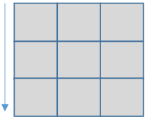
Daily feature extraction: To extract daily features in 2D-CNNpred, 1×number of initial features filters are utilized. Each of those filters covers all the daily features and can combine them into a single higher level feature, so using this layer, 2D-CNNpred can construct different combinations of primary features. It is also possible for the network to drop useless features by setting their cor-responding weights in filters equal to zero. So this layer works as an initial feature extraction/feature selection module. Fig 3 represents application of a simple filter on the input data.
Durational feature extraction: While the first layer of 2D-CNNpred extracts features out of primary daily features, the following layers combine extracted features of different days to construct higher level features for aggregating the
available information in certain durations. Like the first layer, these succeeding layers use filters for combining lower level features from their input to higher level ones. 2D-CNNpred uses 3×1 filters in the second layer. Each of those filters covers three consecutive days, a setting that is inspired by the observation that most of the famous candlestick patterns like Three Line Strike and Three Black Crows, try to find meaningful patterns in three consecutive days (Nison, 1994; Bulkowski, 2012; Achelis, 2001). We take this as a sign of the potentially useful information that can be extracted from a time window of three consecutive times unites in the historical data. The third layer is a pooling layer that performs a 2 × 1 max pooling, that is a very common setting for the pooling layers. After this pooling layer and in order to aggregate the information in longer time intervals and construct even more complex features, 2D-CNNpred uses another convolutional layer with 3 × 1 filters followed by a second pooling layer just like
17
| x= | 1 | 4 |
|---|---|---|
| x= | 1 + exp(x) | 4 |
4.2. 3D-CNNpred
Fig 4 shows a graphical visualization of
the data would be represented.
| past days |  |
t-1 | v1,t-1,1 | … |
|
|---|---|---|---|---|---|
| … | v1,t-j,1 | … | |||
| t-j |
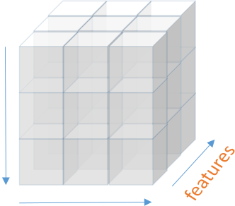
Figure 5: Representation of input data in 3D-CNNpred based on k primary features, i related
markets and j days before the day of prediction
| past days |  |
t-1 | v1,t-1,1 | … |
|
v1,t-1 | … | vj,t-1 |
|---|---|---|---|---|---|---|---|---|
| … | v1,t-j,1 | … |
|
v1,t-i | … | vj,t-i | ||
| t-j | ||||||||
| 1 | … |
Durational feature extraction: In addition to daily features, 3D-CNNpreds input data provides information about other markets. Like 2D-CNNpred, the next four layers are dedicated to extracting higher level features that summarize the fluctuation patterns of the data in time. However, in 3D-CNNpred, this is done over a series of markets instead of one. So, the width of the filters in
20
As we mentioned before, our goal is to develop a model for prediction of the direction of movements of stock market prices or indices. We applied our approach to predict the movement of indices of S&P 500, NASDAQ, Dow Jones Industrial Average, NYSE and RUSSELL market. For this prediction task, we use 82 features for representing each day of each market. Some of these features are market-specific while the rest are general economic features and are replicated for every market in the data set. This rich set of features could be categorized in eight different groups that are primitive features, technical indicators, economic data, world stock market indices, the exchange rate of U.S. dollar to the other currencies, commodities, data from big companies of U.S. market and future contracts. We briefly explain different groups of our feature set here and more details about them can be found in Appendix I.
• Primitive features: Close price and which day of week prediction is sup- posed to happen are primitive features used in this work.
markets. For instance, effect of other countries stock market like China, Japan and South Korea on U.S. market.
• The exchange rate of U.S. dollar: There are companies that import their needs from other countries or export their product to other countries. In these cases, value of U.S. dollar to other currencies like Canadian dollar and European Euro make an important role in the fluctuation of stock prices and by extent, the whole market.
In this section, we describe the settings that are used to evaluate the models, including datasets, parameters of the networks, evaluation methodology and baseline algorithms. Then, the evaluation results are reported.
23
| Name | Description |
|---|
0 Closet+1 > Closet |
(5) |
|---|
24
| Filter size Activation function Optimizer Dropout rate Batch size |
{8, 8, 8} RELU-Sigmoid Adam 0.1 128 |
|---|
Table 3: Parameters of CNN
6.3. Parameters of network
Numerous deep learning packages and software have been developed. In this work, Keras (Chollet et al., 2015) was utilized to implement CNN. The activation function of all the layers except the last one is RELU. Complete descriptions of parameters of CNN are listed in Table 3.
| Simple Moving Average Exponential Moving Average Momentum Stochastic %K Stochastic %D Relative Strength Index Moving Average Convergence Divergence Larry Williams %R (Accumulation\Distribution) Oscillator Commodity Channel Index |
|---|
Table 4: Technical Indicators
• The first baseline algorithm is the one reported in (Zhong & Enke, 2017). In this algorithm, the initial data is mapped to a new feature space using PCA and then the resulting representation of the data is used for training a shallow ANN for making predictions.
26
| 3D-CNNpred 2D-CNNpred PCA+ANN (Zhong & Enke, 2017) Technical (Kara et al., 2011) CNN-cor (Gunduz et al., 2017) |
Our method Our method PCA as dimension reduction and ANN as classifier Technical indicators and ANN as classifier A CNN with mentioned structure in the paper |
|---|
Table 5: Description of used algorithms
It is obvious from the results that both 2D-CNNpred and 3D-CNNpred sta-tistically outperformed the other baseline algorithms. The difference between F-measure of our model and baseline algorithm which uses only ten technical indicators is obvious. A plausible reason for that could be related to the insuf-ficiency of technical indicators for prediction as well as using a shallow ANN
27
| Mean of F-measure Best of F-measure Standard deviation of F-measure P-value against 2D-CNNpred P-value against 3D-CNNpred |
0.003 |
0.3928 |
0.4237 0.5165 |
0.5504 0.0273 |
0.0343 0.5903 |
|---|
| Mean of F-measure Best of F-measure Standard deviation of F-measure P-value against 2D-CNNpred P-value against 3D-CNNpred |
0.0625 less than 0.0001 |
less than 0.0001 less than 0.0001 |
less than 0.0001 |
0.4822 |
0.4925 0.5778 |
|---|
rithms
| Mean of F-measure Best of F-measure Standard deviation of F-measure P-value against 2D-CNNpred P-value against 3D-CNNpred |
0.4199 |
0.3796 0.5498 |
0.5312 0.0553 |
0.0255 1 |
0.0509 1 |
|---|
| Mean of F-measure Best of F-measure Standard deviation of F-measure P-value against 2D-CNNpred P-value against 3D-CNNpred |
0.0556 less than 0.0001 |
less than 0.0001 less than 0.0001 |
less than 0.0001 |
0.4757 |
0.4751 0.5592 |
|---|
| Mean of F-measure Best of F-measure Standard deviation of F-measure P-value against 2D-CNNpred P-value against 3D-CNNpred |
0.4525 0.5665 |
0.5602 0.0977 |
0.066 0.0001 |
1 0.3364 |
1 |
|---|
Table 10: Statistical information of RUSSELL 2000 using different algorithms
|
2D-CNNpred |
|
|||||
|---|---|---|---|---|---|---|---|
| 44.69 | 39.28 | 42.37 | 47.99 | ||||
PCA+ANN Technical CNN-Cor |
|||||||
| Mean F-measure | 45 | ||||||
| 43 | |||||||
| S&P 500 | DJI |
|
|
||||
30
among all the tested algorithms. CNNs ability in feature extraction is highly dependent on wisely selection of its parameters in a way that fits the problem for which it is supposed to be applied. With regards to the fact that both 2D-CNNpred and CNN-Cor used the same feature set and they were trained almost in the same way, poor results of CNN-Cor compared to 2D-CNNpred is possibly the result of the design of the 2D-CNN. Generally, the idea of using 3 × 3 and 5 × 5 filters seems skeptical. The fact that these kinds of filters are popular in computer vision does not guarantee that they would work well in stock market prediction as well. In fact, prediction with about 9% lower F-measure on average in comparison to the 2D-CNNpred showed that designing the structure of CNN is the core challenge in applying CNNs for stock market prediction. A poorly designed CNN can adversely influence the results and make CNNs performance even worse than a shallow ANN.
31
gorithms. CNNpred was able to improve the performance of prediction in all the five indices over the baseline algorithms by about 3% to 11%, in terms of F-measure. In addition to confirming the usefulness of the suggested approach, these observations also suggest that designing the structures of CNNs for the stock prediction problems is possibly a core challenge that deserves to be further studied.
33 34 |
CTB1Y
|
Economic
|
|
|---|
33
| FCHI FTSE GDAXI USD-Y USD-GBP USD-CAD USD-CNY USD-AUD USD-NZD USD-CHF USD-EUR USDX XOM JPM AAPL MSFT GE JNJ WFC AMZN FCHI-F FTSE-F GDAXI-F HSI-F Nikkei-F KOSPI-F IXIC-F DJI-F S&P-F RUSSELL-F USDX-F |
|
|
|---|
Achelis, S. B. (2001). Technical Analysis from A to Z. McGraw Hill New York.
Ar´evalo, A., Ni˜no, J., Hern´andez, G., & Sandoval, J. (2016). High-frequency trading strategy based on deep neural networks. In International conference on intelligent computing (pp. 424–436). Springer.
classifiers for stock price direction prediction. Expert Systems with Applications, 42, 7046–7056.
Bao, W., Yue, J., & Rao, Y. (2017). A deep learning framework for financial time series using stacked autoencoders and long-short term memory. PloS one, 12, e0180944.
Chollet, F. et al. (2015). Keras. .
Chong, E., Han, C., & Park, F. C. (2017). Deep learning networks for stock market analysis and prediction: Methodology, data representations, and case studies. Expert Systems with Applications, 83, 187–205.
Gardner, M. W., & Dorling, S. (1998). Artificial neural networks (the multilayer perceptron)a review of applications in the atmospheric sciences. Atmospheric envi- ronment, 32, 2627–2636.
Gunduz, H., Yaslan, Y., & Cataltepe, Z. (2017). Intraday prediction of borsa istan-bul using convolutional neural networks and feature correlations. Knowledge-Based Systems, 137, 138–148.
Hinton, G. E., Srivastava, N., Krizhevsky, A., Sutskever, I., & Salakhutdinov, R. R. (2012). Improving neural networks by preventing co-adaptation of feature detectors. arXiv preprint arXiv:1207.0580, .
Hu, Y., Feng, B., Zhang, X., Ngai, E., & Liu, M. (2015a). Stock trading rule discovery with an evolutionary trend following model. Expert Systems with Applications, 42, 212–222.
Kim, K.-j. (2003). Financial time series forecasting using support vector machines. Neurocomputing, 55, 307–319.
Kim, K.-j., & Han, I. (2000). Genetic algorithms approach to feature discretization in artificial neural networks for the prediction of stock price index. Expert systems with Applications, 19, 125–132.
Moghaddam, A. H., Moghaddam, M. H., & Esfandyari, M. (2016). Stock market
index prediction using artificial neural network. and Administrative Science, 21, 89–93.
Nelson, D. M., Pereira, A. C., & de Oliveira, R. A. (2017). Stock market’s price movement prediction with lstm neural networks. In Neural Networks (IJCNN), 2017 International Joint Conference on (pp. 1419–1426). IEEE.
Nison, S. (1994). Beyond candlesticks: New Japanese charting techniques revealed volume 56. John Wiley & Sons.
Qiu, M., & Song, Y. (2016). Predicting the direction of stock market index movement using an optimized artificial neural network model. PloS one, 11, e0155133.
Qiu, M., Song, Y., & Akagi, F. (2016). Application of artificial neural network for the prediction of stock market returns: The case of the japanese stock market. Chaos, Solitons & Fractals, 85, 1–7.
Zhang, Y., & Wu, L. (2009). Stock market prediction of s&p 500 via combination of improved bco approach and bp neural network. Expert systems with applications, 36, 8849–8854.
Zhao, Y., Li, J., & Yu, L. (2017). A deep learning ensemble approach for crude oil price forecasting. Energy Economics, 66, 9–16.