
Trobe universityillustrations and web design catherine tan
Integration
Integration – A guide for teachers (Years 11–12)
Full bibliographic details are available from Education Services Australia.
Published by Education Services Australia
PO Box 177
Carlton South Vic 3053
Australia
Australian Mathematical Sciences Institute
Building 161
The University of Melbourne
VIC 3010
Email: enquiries@amsi.org.au
Website: www.amsi.org.au
History and applications . . . . . . . . . . . . . . . . . . . . . . . . . . . . . . . . . . . 31
Appendix . . . . . . . . . . . . . . . . . . . . . . . . . . . . . . . . . . . . . . . . . . . . 34 A comparison of area estimates, and Simpson’s rule . . . . . . . . . . . . . . . . . 34 Exactness of area estimates . . . . . . . . . . . . . . . . . . . . . . . . . . . . . . . . 35 Functions integrable and not . . . . . . . . . . . . . . . . . . . . . . . . . . . . . . . 36
Assumed knowledge
• The content of the module Introduction to differential calculus.
Adding up a function in small pieces
You ride your bicycle for 5 minutes. Your bike is equipped with a fancy speedometer, and
speedometer said otherwise!
| ∆ t | t |
|---|
mate for how far you went over the whole 5 minutes.
A guide for teachers – Years 11 and 12 • {5}
We’ve previously seen differentiation, and you might recall that differentiation can an-swer a related question. If you know where you are on your bike (i.e., your displacement) at every instant, then you can work out your velocity at every instant. If f (t) is how far you’ve travelled at time t, then the derivative f′(t) gives your instantaneous velocity at time t. This is the opposite problem: given position, we used differentiation to figure out velocity; now, given velocity, we use integration to figure out position.
1 If you tried to perform these calculations while on your bike, you likely would have crashed it. If you kept your eye on your speedometer at every instant, you certainly would have crashed it!
Calculus is a crucial area of mathematics, necessary for understanding how quantities change in relation to each other, and for understanding almost every aspect of the phys-ical world. Differentiation deals with how one quantity changes with respect to another, in the limit of small changes. But it is only half the story. Integration deals with the sum of these small changes, in the limit, adding them up and putting them back together again. Whether it’s your speed on your bike, or biological populations, or chemical concentra-tions, or economic indicators, or environmental conditions, or physical phenomena —to understand how quantities in the world are related, we need to understand both dif-ferential and integral calculus.
Other questions
A guide for teachers – Years 11 and 12 • {7}
Content
The area under a graph
| 0 | x | 5 |
|---|
As a first approximation, we can divide the interval [0,5] into five subintervals of width 1, i.e., [0,1], [1,2], ..., [4,5], and consider rectangles as shown on the following graph.
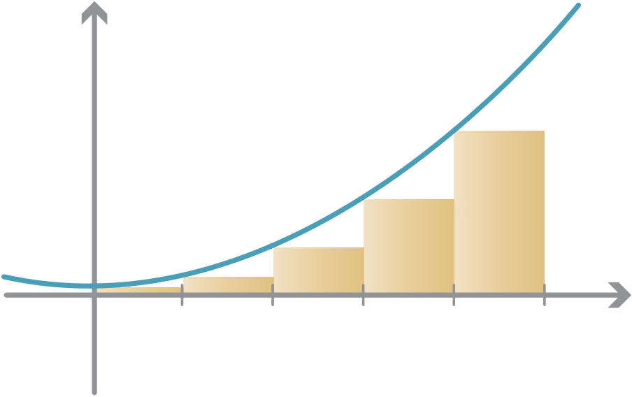
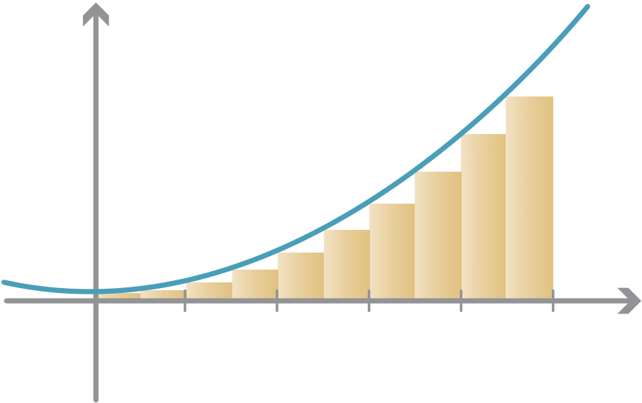
Approximating the area under the graph with 5 rectangles
| Interval | Width of rectangle | Height of rectangle | Area of rectangle |
|---|---|---|---|
| [0,1] | 1 | f (0) = 02+1 = 1 | 1 |
| [1,2] | 1 | f (1) = 12+1 = 2 | 2 |
| [2,3] | 1 | f (2) = 22+1 = 5 | 5 |
| [3,4] | 1 | f (3) = 32+1 = 10 | 10 |
| [4,5] | 1 | f (4) = 42+1 = 17 | 17 |
| 35 | |||
| Total area |
For a slightly better approximation, we can split the interval into 10 equal subintervals, each of length1 2. Using the same idea, we have the rectangles shown on the following graph. We clearly have a better estimate, but still an underestimate.
| Interval | Width of rectangle | Height of rectangle | Area of rectangle |
|---|---|---|---|
| [0,1 2] | 1 | f (0) = 0+1 = 1 | 1 |
| 2 | 2 | ||
| [1 2,1] | 1 | f (1 2) = |
5 |
| 2 | 8 | ||
| [1,3 2] | 1 | f (1) = 1+1 = 2 | 1 |
| 2 | |||
| [3 2,2] | 1 | f (3 2) = |
13 |
| 2 | 8 | ||
| [2,5 2] | 1 | f (2) = 4+1 = 5 | 5 |
| 2 | 2 | ||
| [5 2,3] | 1 | f (5 2) = |
29 |
| 2 | 8 | ||
| [3,7 2] | 1 | f (3) = 9+1 = 10 | 5 |
| 2 | |||
| [7 2,4] | 1 | f (7 2) = |
53 |
| 2 | 8 | ||
| [4,9 2] | 1 | f (4) = 16+1 = 17 | 17 |
| 2 | 2 | ||
| [9 2,5] | 1 | f (9 2) = |
85 |
| 2 | 8 | ||
|
|||
| Total area |
Splitting [0,5] into more subintervals of smaller width, we can perform the same calcula-tion and estimate the area. With more rectangles, the calculations become more tedious, but some results are given in the following table.
{10} • Integration
Estimates of area
As the numbers are equally spaced, the width of each interval is1 n(b − a). That is, x j − x j−1 =b − a , for all j = 1,2,...,n.
We also write ∆x for this width, the ‘change in x’ between successive endpoints.
| x j = a + j | �b − a | � |
|---|
Above the interval [x0,x1], we have a rectangle whose width is ∆x and whose height is f (x0). In general, above the interval [x j−1,x j], we have a rectangle of width ∆x and height f (x j−1). The area of this rectangle is then f (x j−1) ∆x. The total area estimate is therefore
| � | f (x1)+ f (x2)+···+ f (xn)� | ∆x = | j=1 n� |
|---|
A guide for teachers – Years 11 and 12 • {11}
| Midpoint estimate. |
|---|
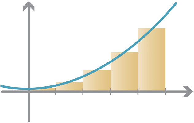
Estimate the area under the graph of y = x3between 0 and 2, using the right-endpoint
|
|---|
{12} • Integration
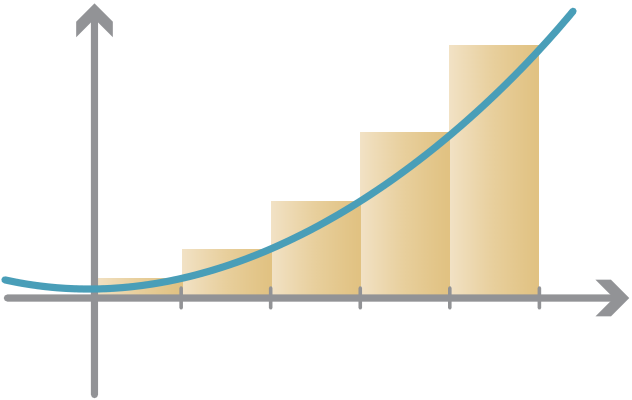
Estimate the area under the graph of y = x2+ x between x = 0 and x = 4, using the mid-point estimate with two subintervals.
Exercise 3
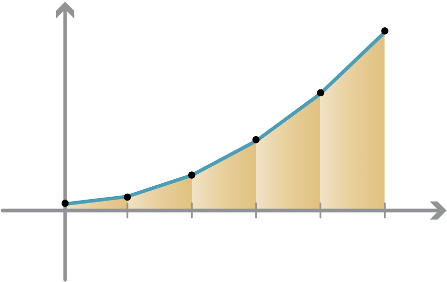
We need not restrict ourselves to rectangles. Instead, we could plot the points on the
graph y = f (x) for each x j, and join the dots. In this way, the function f (x) is approxi-mated by a piecewise linear function, that is, a sequence of straight line segments. The
| 0 | 1 | 2 | 3 | 4 | 5 |
|---|
A guide for teachers – Years 11 and 12 • {13}
right-endpoint estimate.
Limits of estimates
Dividing the interval [0,1] into n subintervals
|
y | y = f(x) | ||
|---|---|---|---|---|
| ∆x =1 | and | |||
{14} • Integration
As it turns out, there is a formula for the sum of the first n squares:
| j=1 n� | j2= 12+22+···+n2=n(n +1)(2n +1) |
|---|
| j=1 n� | j = 1+2+···+n =n(n +1) |
|---|
calculate the right-endpoint estimate for the area under the graph y = x between x = 0 and x = 1. Take the limit as n → ∞ to find the exact area. Confirm your answer using elementary geometry.
Definition of the integral
For a function f (x), considered between x = a and x = b, the limit we obtain for the exact area is denoted by
�b f (x) dx
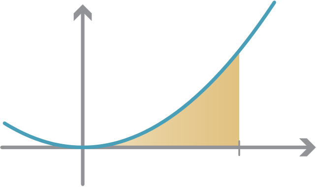
Let’s return to our function f (x) = x2+1, and our quest to find the area under the graph y = f (x) between x = 0 and x = 5, i.e.,
�5 (x2+1) dx.
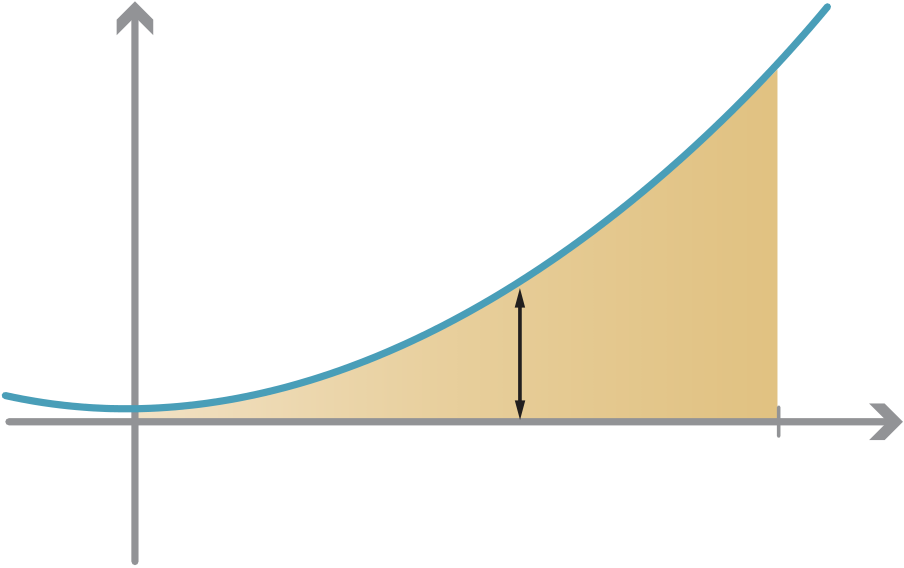
To calculate the exact area, we introduce an area function A. For any fixed number c > 0, let A(c) be the area under the graph y = f (x) between x = 0 and x = c. So we can define the function A(x) to be the area between 0 and x. Clearly A(0) = 0. We seek A(5).
A(x)
| 0 | x |
|---|
{16} • Integration
In fact, A′(x) = f (x). We can see this geometrically. To differentiate A(x) from first prin-ciples, we consider
| y | y = f(x) |
|---|
If you were to ‘level off’ the area under the graph between x and x + h, you’d obtain a rectangle (as shown in the graph above) with width h and height equal to the average
| area of rectangle | ||
|---|---|---|
| h | = | width of rectangle |
If h becomes very small, then the interval [x,x + h] approaches the single point x. And the average value of f over this interval must approach f (x). So we have
Returning again to our example f (x) = x2+ 1, what then is the area function A(x)? Its derivative must be f (x) = x2+1. We’re looking for a function A such that
|
and |
|---|
satisfies these criteria. Hence the total area is
A(5) =125 3+5 = 140 = 462 3,
Importantly, antiderivatives are not unique. A given function can have many antideriva-tives. For instance, the following functions are all antiderivatives of x2:
|
|
|---|
{18} • Integration
Exercise 6
| Function | General antiderivative |
|
|---|---|---|
| xn |
|
|
| (ax +b)n | for a,b,c,n any real constants with a ̸= 0, n ̸= −1 |
|
|---|
The following theorem gives some useful rules for computing integrals.
�k f (x) dx = k�f (x) dx.
This theorem allows us to compute an antiderivative by treating a function term-by-term
= 3�x3dx −4�x2dx +2�1 dx =3x4 4− 4x3 3+2x +c. |
Exercise 8
Find
A general method to find the area under a graph y = f (x) between x = a and x = b is given by the following important theorem.
Theorem (Fundamental theorem of calculus)
| �b | f (x) dx = |
|---|
subtract; it is synonymous with F(b)−F(a).�F(x)�b ais just a shorthand to substitute x = a and x = b into F(x) and
Note that any antiderivative of f (x) will work in the above theorem. Indeed, if we have
We give a proof of the theorem, assuming our previous statements:
Proof
As before, let A(c) be the area under the
| y | y = f(x) |
|---|
tiderivatives of f (x), they must differ by
a constant, i.e., A(x) = F(x)+K for some constant K . Since A(a) = 0, this implies F(a) +K = 0. Hence K = −F(a), and it follows that A(x) = F(x) −F(a). Therefore the desired integral is equal to A(b) = F(b)−F(a).
Find
| �8 | (3x2+ | 3� |
|
|---|
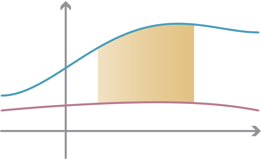
Our idea of estimating your distance travelled by breaking your trip up into 1-minute intervals is nothing more than an area estimate. We may divide the time interval [a,b] into n subintervals [t0,t1],[t1,t2],...,[tn−1,tn], each of width ∆t =1 n(b − a). We can esti-mate your velocity over the interval [t j−1,t j] by the constant v(t j) (i.e., using the right-endpoint estimate); over this interval of time, you travelled a distance of approximately v(t j) ∆t. The total distance travelled, then, is approximately
j=1 n�v(t j) ∆t.
The right-endpoint estimate for area under y = v(t) estimates displacement.
In the limit, as we take more and more shorter and shorter time intervals, we obtain the exact change in position (displacement) as
�b v(t) dt.
A guide for teachers – Years 11 and 12 • {23}
Areas above and below the axis
| a |
|
0 |
|
– | + |
|---|
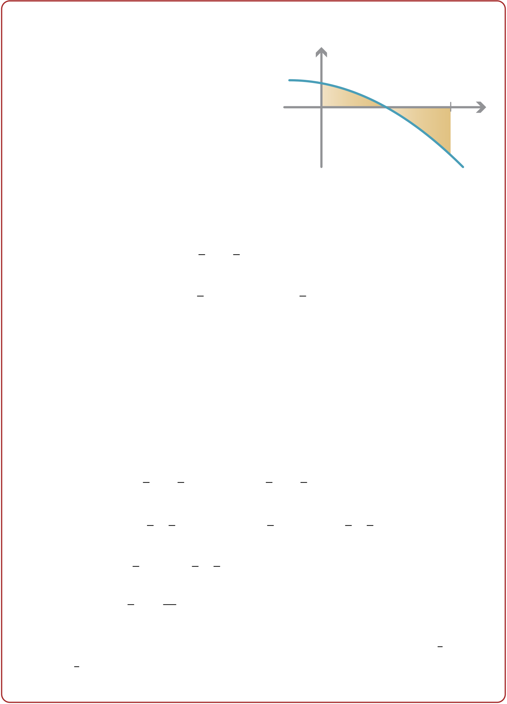
In general, to find the total area enclosed between a graph and the axis, we find where the graph crosses the axis and compute the areas separately. See the following example.
Solution
1 |
�2 | (−x2− x +2) dx = | �−1 3x3 − 1 2x2 +2x | |||
|---|---|---|---|---|---|---|
| = | �−8 3−2+4� | − | = −2 3. | |||
|
||||||
−x2− x +2 = −(x −1)(x +2),
signs, as in the above example! It is good practice to carefully bracket all terms, as shown.
y = x + 1
x
–2 0 2Definite integrals obey rules similar to those for indefinite integrals. The following theo-
rem is analogous to one for indefinite integrals.
| �b | � | f (x)± g(x)� | dx = | �b | f (x) dx ± | �b |
|
||
|---|---|---|---|---|---|---|---|---|---|
|
|||||||||
| �b | k f (x) dx = k | �b | |||||||
{26} • Integration
Exercise 13
Find a geometric interpretation of part (b) of the first theorem of this section (linearity of integration). You may assume the graph of y = f (x) lies above the x-axis. Also find an interpretation in terms of antiderivatives.
| �b | f (x) dx = − | �a |
|---|
|
|||
|---|---|---|---|
| �b | |||
| Find | �0 | ||
|
|||
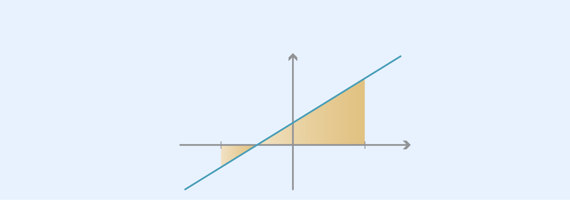
This formula works regardless of whether the graphs are above or below the x-axis, as
long as the graph of f (x) is above the graph of g(x). (Can you see why?)
integrals of f (x)− g(x) or g(x)− f (x) respectively.
Example
| 0 | 2 | x |
|---|
{28} • Integration
|
|---|
A guide for teachers – Years 11 and 12 • {29}
has rotational symmetry about the x-axis and is called a solid of revolution.
| z |
|
x | z | y |
|
x |
|---|
More generally, if we have a solid bounded by the two parallel planes x = a and x = b, and at each value of x in [a,b] the cross-sectional area of the solid is A(x), then the volume of
the solid is
Arc length
How long is a piece of string? If the piece of string is given as a graph y = f (x) then its length can be calculated using integration.
y
∆y
| ∆y | ∆y | 4 | ||||||
|---|---|---|---|---|---|---|---|---|
| ∆y | 1 | |||||||
| 0 | ∆x | 1 | 2 | 3 | ||||
|
||||||||
Difficulties with antiderivatives
finding antiderivatives, there are no rules as simple as the product, chain and quotient rules for differentiation.
For an interesting and important example, consider the function f : R → R defined by f (x) = e−x2.
|
|---|
2 Lord Kelvin, the mathematical physicist and engineer, once joked that a mathematician is a person for whom this equation is as obvious as the equation 2+2 = 4 is to the average person!
�1−1 (1− x2) dx.
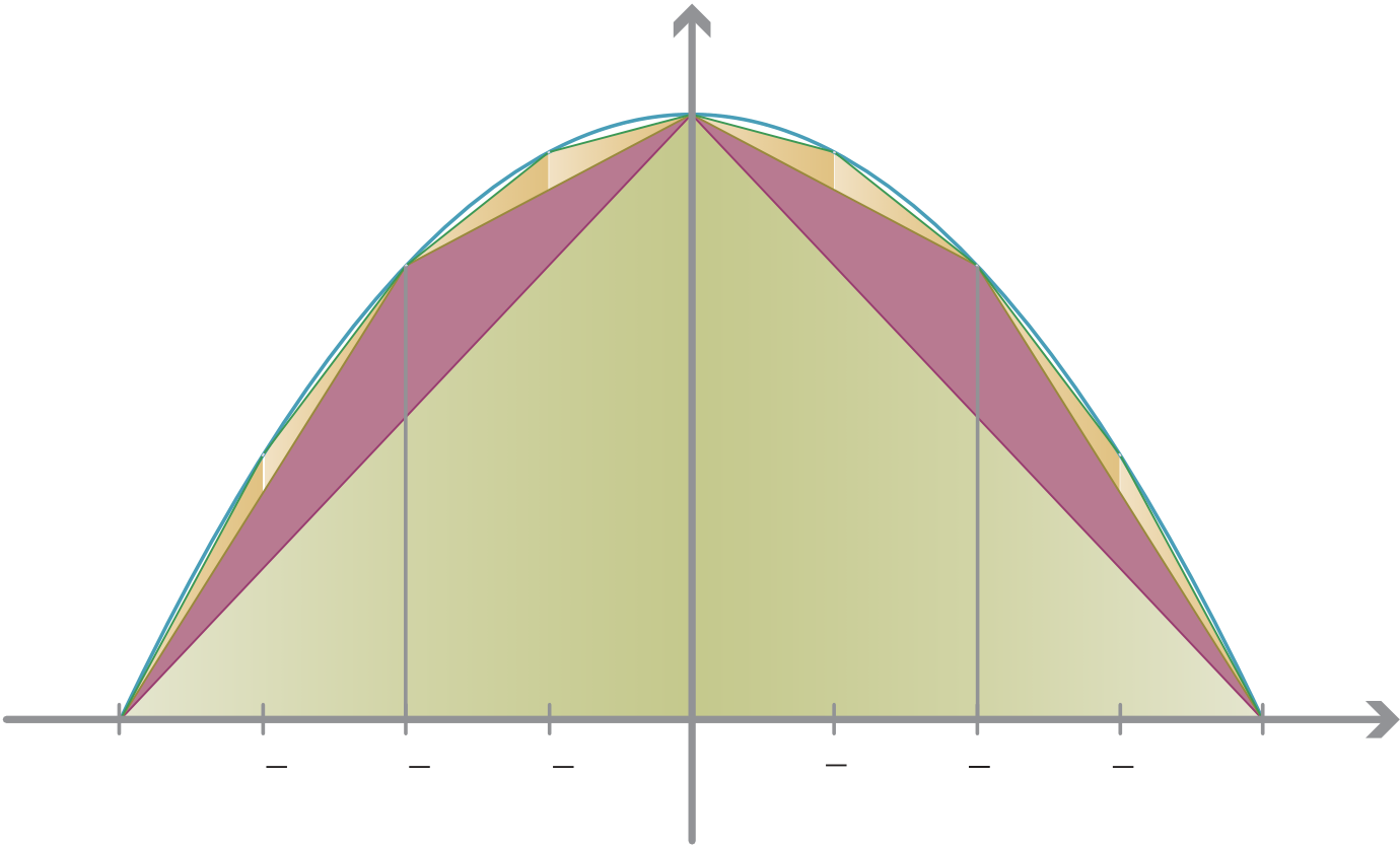
It’s interesting to compare our ‘modern’ (17th century CE) technique to Archimedes’. We would compute this area as
| A | – |
|
G | – |
|
M | H | 1 | x | |||||
|---|---|---|---|---|---|---|---|---|---|---|---|---|---|---|
| F | ||||||||||||||
| D | E |
|
||||||||||||
| – |
|
|||||||||||||
| –1 | ||||||||||||||
As we proceed, we inscribe more and more triangles inside the parabola. In the next step we inscribe four triangles, after that we inscribe eight triangles. At the nth stage, we inscribe 2ntriangles in the gaps between previous triangles. Archimedes was able to show that, at each stage, the triangles all have half the width and a quarter the height of the triangles from the previous stage, and hence an eighth the area.
A comparison of area estimates, and Simpson’s rule
We have mentioned several different ways of estimating the area under a curve: left-
All of the estimates discussed give the approximate area under y = f (x) in the form of
a sum of products of values of f with the width ∆x. In fact, the left-endpoint, right-
|
c0 | c1 | c2 | c3 | c4 | ... | cn−2 | cn−1 | cn |
|---|---|---|---|---|---|---|---|---|---|
|
1 | 1 | 1 | 1 | 1 | ... | 1 | 1 | 0 |
| right endpoint | 0 | 1 | 1 | 1 | 1 | ... | 1 | 1 | 1 |
| 1 | 1 | 1 | 1 | 1 | ... | 1 | 1 | 1 | |
| 2 | 2 | ||||||||
| 1 | 4 | 2 | 4 | 2 | ... | 2 | 4 | 1 | |
| 3 | 3 | 3 | 3 | 3 | 3 | 3 | 3 |
The coefficients start at1 3, then alternate between
4 3and2 3, before ending again at1 3.(It is as if every second coefficient in the list for the trapezoidal estimate donated1 6to
Although the coefficients may appear somewhat bizarre, Simpson’s rule almost always
gives a much more accurate answer than any of the other estimates mentioned. We’ll see
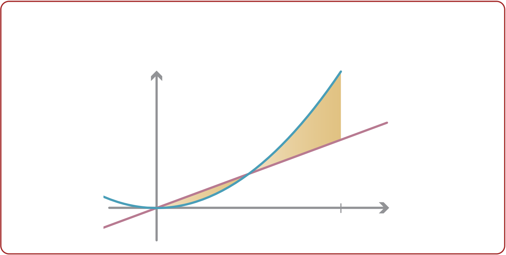
Consider some simple functions f (x) — constant, linear, quadratic — and see how the various estimates fare in approximating the integral�b af (x) dx.
First suppose f (x) is a constant function. In this case, we obtain an exactly correct an-swer for the area under the graph from the left-endpoint, right-endpoint, midpoint or trapezoidal estimate. The area under y = f (x) is itself a rectangle; breaking it up into rectangles or trapezia, we still have the exactly correct area. This is true regardless of the number of subintervals n: we could split [a,b] into just one subinterval, or a million; in all cases we obtain the exactly correct answer.
Next suppose f (x) is a (non-constant) linear function. In this case the left- and right-endpoint estimates will definitely not give you the correct answer. However, the mid-point and trapezoidal estimates will give you the exactly correct answer. The midpoint estimate builds rectangles which have exactly the same amount of area above and below the line. And breaking the area under y = f (x) into trapezia gives the exactly correct area. Again this is true whatever number of subintervals we take.
However, when f (x) is a quadratic function, in general none of the left-endpoint, right-endpoint, midpoint or trapezoidal estimates will give the correct area. Let’s consider the function f (x) = x2, and see how the midpoint and trapezoidal estimates fare. We’ll just take one subinterval, n = 1, so ∆x = b − a.
| M = f | �a +b | � | ∆x = | �1 4a2 + 1 2ab + 1 4b2��b − a |
|---|
{36} • Integration
The correct answer, on the other hand, is
| �b | x2dx = | �x3 | �b | =1 3b3 − 1 3a3 = 1 | � | a2+ ab +b2��b − a |
|---|
This combination of the midpoint and trapezoidal rules will in fact give us an exactly correct answer for the integral of any quadratic function.
| 3M + 1 3T = | �b − a | � | |||
|---|---|---|---|---|---|
| +1 3f (b) |
|
||||
| =b − a | |||||
This pattern of coefficients1 3,
4 3,1 3is exactly Simpson’s rule with two subintervals; if we take1 3(2M+T ) for the midpoint and trapezoidal estimates with n subintervals, we obtain Simpson’s rule with 2n subintervals.
A guide for teachers – Years 11 and 12 • {37}
Riemann integration works for any function f : [a,b] → R that is continuous — roughly, when the graph y = f (x) can be drawn without taking your pen off the paper. It also works for any piecewise continuous function — where you may take your pen off the paper, but only a finite number of times.
if x is irrational.
ber arbitrarily close, and there is an irrational number arbitrarily close. So f (x) is discon-tinuous at every real number x.
x j = (x j − x j−1)+(x j−1 − x j−2)+···+(x1 − x0)+ x0
= j ∆x + x0= a + j ∆x.
Exercise 3
|
|---|
When f is decreasing, we have the opposite inequalities
| f (x j−1) ≥ f | �x j−1 + x j | � |
|
|---|---|---|---|
= trapezoidal estimate.
A guide for teachers – Years 11 and 12 • {39}
| j=1 n� | f (x j) ∆x = | j=1 n� | f | � j n | � 1 n= | j=1 n� | � j n | � 1 n= 1 n2 | j=1 n� | ||||
|---|---|---|---|---|---|---|---|---|---|---|---|---|---|
|
|||||||||||||
| 1 | � | ||||||||||||
| 2 | � | ||||||||||||
|
|||||||||||||
can confirm that its area is1 2·1·1 =
1 2.b Rewriting as obtain �(−2x + 3)−2dx, the integrand is again of the form (ax + b)n, and we
1 1
2(−2x +3)−1 +c = 2(3−2x)+c.
| b | |||||||||
|---|---|---|---|---|---|---|---|---|---|
|
33 | 4 | 8 | 3 | |||||
| �x+ 4x | 3 | � | = | �512+ 4·16� | − | �0+0� |
|
||
| �1 4x4 − 1 2x2 | �2−2 |
|
|||
|---|---|---|---|---|---|
| a | �2−2 | (x3− x) dx = | |||
| b |
�−�1 4− 1�=1 4,
|
||||
Exercise 13
The equation
�b ak f (x) dx =�kF(x)�b a= kF(b)−kF(a) = k�F(x)�b a= k�b af (x) dx.
Exercise 14
wards from 5 to 0; so the answer should be positive.
| 0 | 1 | 2 | 3 | 4 | 5 | 6 | 7 | 8 | 9 | 10 | 11 |
|---|