Write a MATLAB Program

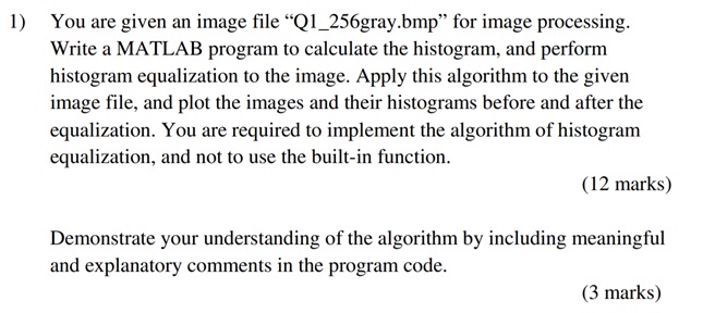
image=imread('Q1_256gray.bmp');% read image

%calculate image histogram

hist_1=zeros(256,1);

for i=1:size(image,1)

    for j=1:size(image,2)

        hist_1(image(i,j)+1)=hist_1(image(i,j)+1)+1;

    end

end

result=[];

temp=0;

%calculate histogram equalization

for i=1:256

    temp=hist_1(i)+temp;

    result(i)=round((temp/(size(image,1)*size(image,2)))*255);

end

image_result=[];

%calculate result image

for i=1:size(image,1)

    for j=1:size(image,2)

        image_result(i,j)=result(image(i,j)+1);

    end

end

hist_2=zeros(256,1);

for i=1:size(image,1)

    for j=1:size(image,2)

        hist_2(image_result(i,j)+1)=hist_2(image_result(i,j)+1)+1;

    end

end

image_result=mat2gray(image_result);

%show all images

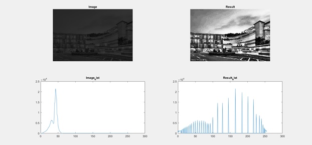
subplot(2,2,1);

imshow(image);

title('Image');

subplot(2,2,3);

plot(0:1:255,hist_1);

title('Image_hist');

subplot(2,2,2);

imshow(image_result);

title('Result');

subplot(2,2,4);

plot(0:1:255,hist_2);

title('Result_hist');

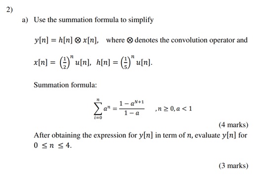
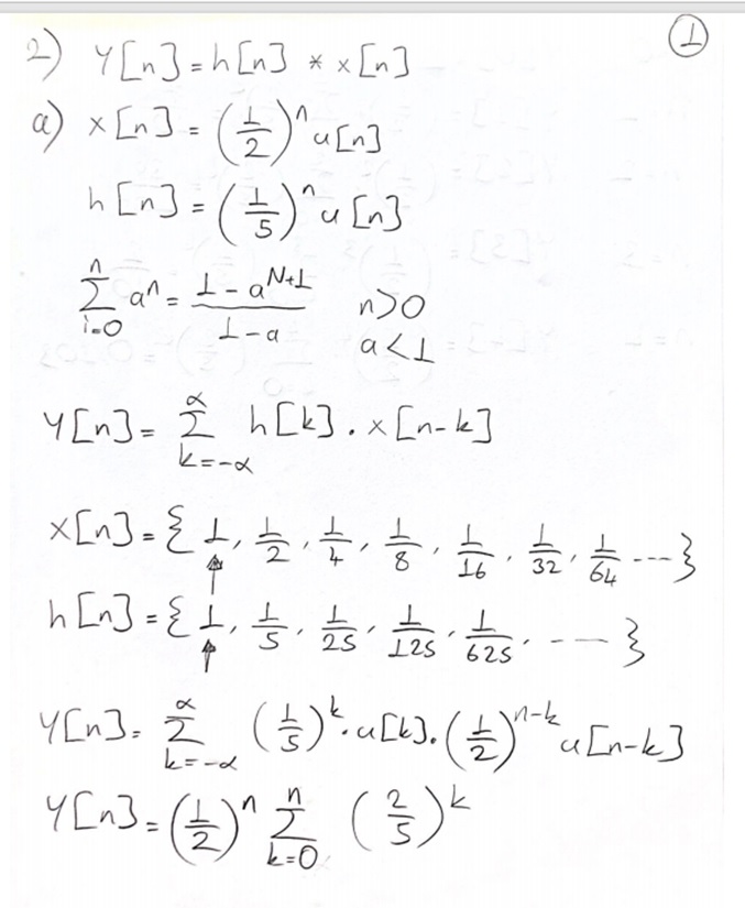
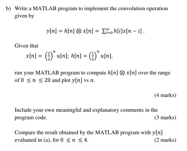
n=0:20;

x = (1/2).^n;

h = (1/5).^n;

y = zeros(1,41);

for i=1:21

    for j=1:21

        y(i+j-1) =  y(i+j-1) + x(i)*h(j);

    end

   

end

stem(n,y(n+1))

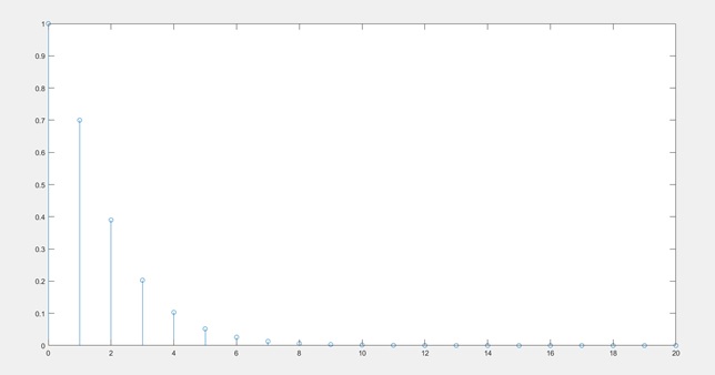
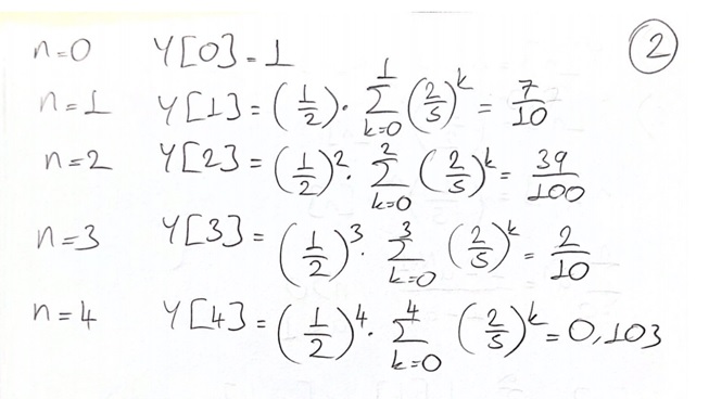
Comparision

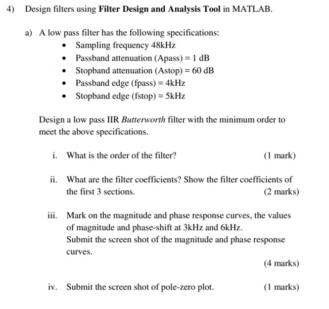
Fs  = 48e3;

Fp  = 4e3/Fs;

Fp_1  = 5e3/Fs;

Ap  = 1;

Ast = 60;

N = 1;

F3dB = 0.09375;

d = fdesign.lowpass('N,F3dB',N,F3dB);

setspecs(d,'Fp,Fst,Ap,Ast',Fp,Fp_1,Ap,Ast);

Hbutter = design(d,'butter','SystemObject',true);

hfvt = fvtool(Hbutter, 'DesignMask', 'on','Color','white');

axis([0 1 -70 2])

legend(hfvt,  'Butterworth');

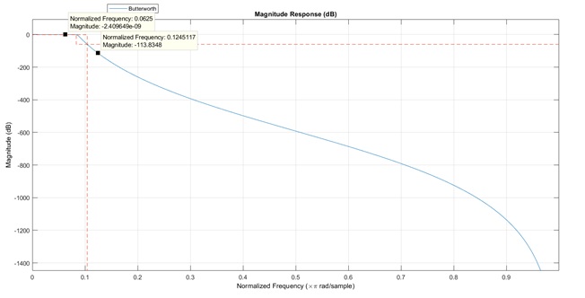
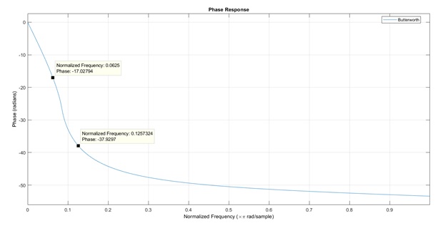
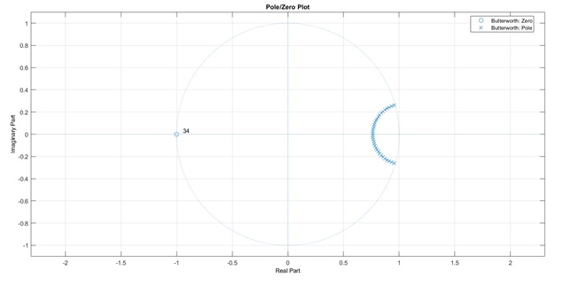
• Minimum order is 34

Magnitude

Phase

Fs  = 48e3;

Fp  = 4e3/Fs;

Fp_1  = 5e3/Fs;

Ap  = 1;

Ast = 60;

N = 1;

F3dB = 0.09375;

d = fdesign.lowpass('N,F3dB',N,F3dB);

setspecs(d,'Fp,Fst,Ap,Ast',Fp,Fp_1,Ap,Ast);

Hbutter = design(d,'cheby2','SystemObject',true);

hfvt = fvtool(Hbutter, 'DesignMask', 'on','Color','white');

legend(hfvt,  'Butterworth');

• Minimum order is 12

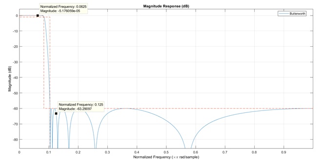
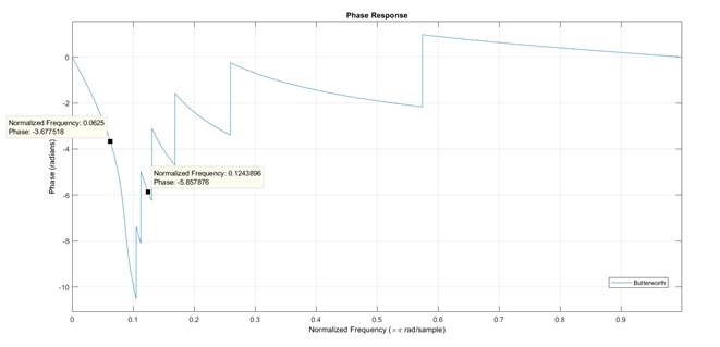
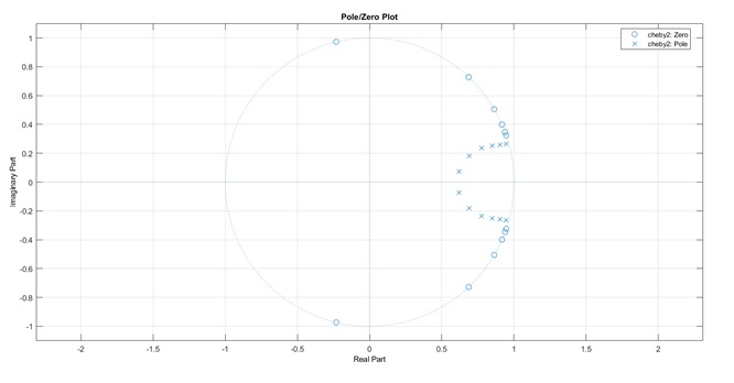
We can see that the order of butterworth filter is higher than Chebyshev filter. So there are less multiplication for calculating. But butterworth filter’s phase response is smoother than Chebyshev filter.

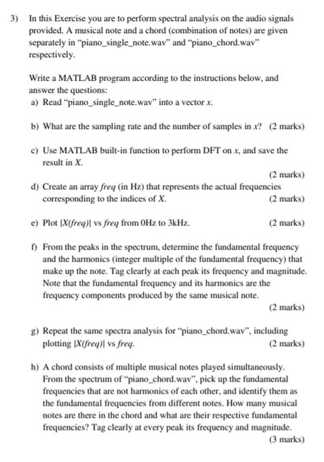
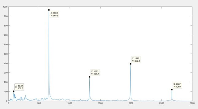
1. [x,Fs]=audioread("piano_single_note.wav");
2. Fs = 44100 Hz
3. X = fft(x,length(x));
4. freq = Fs*(0:length(X)-1)/(length(X));
5. plot(freq,abs(X));

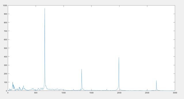
xlim([0 3000])

1. frequencies; 86.61 , 660.6, 1323, 1992, 2667

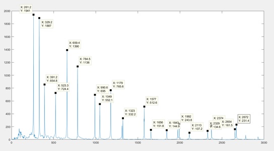
2. [x,Fs]=audioread("piano_chord.wav");

X = fft(x,length(x));

freq = Fs*(0:length(X)-1)/(length(X));

plot(freq,abs(X));

xlim([0 3000])

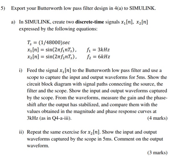
X1

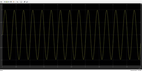
X2

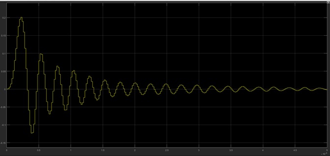
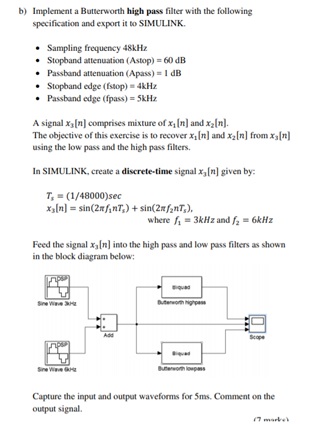
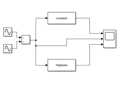
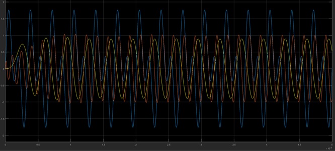
X1 signal is passing though low pass filter without any attenuation, but X2 signal is attenuating because of its frequency.

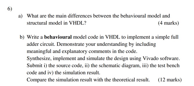
a) difference between behavioral and structural code in VHDL

in structural modeling uses gates and other primitives for defining the design circuit.

In behavioral modeling uses switch-case, for/while loop, if-else for defining the hardware

b)

LIBRARY ieee;

USE ieee.std_logic_1164.ALL;

ENTITY test_adder IS

END test_adder;

ARCHITECTURE behavior OF test_adder IS

COMPONENT adder_code

PORT(

A1 : IN std_logic;

A2 : IN std_logic;

Carry_in : IN std_logic;

Sum : OUT std_logic;

Carry_out : OUT std_logic

);

END COMPONENT;

signal Carry_in : std_logic ;

signal A1 : std_logic ;

signal A2 : std_logic;

signal Sum : std_logic;

signal Carry_out : std_logic;

BEGIN

uut: adder_code PORT MAP (

A1 => A1,

A2 => A2,

Carry_in => Carry_in,

Sum => Sum,

Cout => Cout

);

stim_proc: process

begin

wait for 1 ns;

A1 <= '1';

A2<= '0';

Carry_in <= '0';

wait for 1 ns;

A1 <= '0';

A2<= '1';

Carry_in <= '0';

wait for 1 ns;

A1 <= '1';

A2<= '0';

Carry_in <= '1';

end process;

END;

The code:

entity adder_code is

Port ( A1 : in STD_LOGIC;

A2 : in STD_LOGIC;

Carry_in : in STD_LOGIC;

Sum : out STD_LOGIC;

Carry_out : out STD_LOGIC);

end adder_code;

architecture adder of adder_code is

begin

process(A1,A2,Carry_in)

begin

Cout <= (A1 AND A2) OR (Carry_in AND A1) OR (Carry_in AND A2) ;

Sum <= A1 XOR A2 XOR Carry_in ;

end process;

end adder;