Data Analytics Assignment Help

                    Big Data & Business Analytics ATP Men’s Tour 2014 Match
                    Results and Betting Odds
                  

1 Introduction of database and data science techniques

For the following paper we have chosen a database about the ATP World Tour 2014 as all team members possess a keen interest in tennis and therewith it enabled us to verify findings and make a parallel with an expert know - how. Due to many different variables, the group members could decide between various different analyses and were not too limited by the dataset.

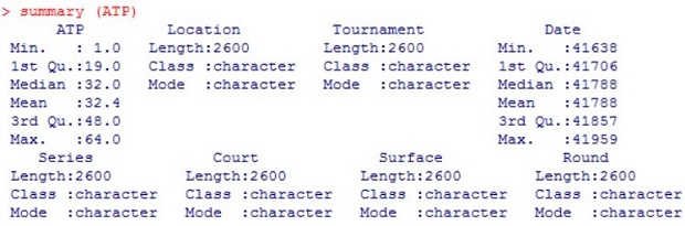
The chosen data set is dealing with the match results and betting odds of the 2014 ATP season. It was provided by tennis - data, combining data from Xscores, ATPtennis, ATP Tour Rankings and Results Page, Livescore and Oddsportal. Furthermore, it includes 2600 instances and a total of 42 variables. Annex 1 gives an overview and explanations about the variables. This works focus especially, among other variables, on the winner ranking (WRank), the average odds of the winner (AvgW) and the winner’s p oints (WPts). The next chapters will present several different analyses, including a correlation analysis, three linear multiple regressions, three decision trees, and a nearest neighbor analysis (including loops). At the end, limitations of the dataset and of the analyses are stated and a conclusion will be drawn.

Before using the dataset in R, we first had to clean it. Several fields were left empty or filled with the term N/A. I n order to use the dataset within R, these fields got coded with 0 to avoid that R interprets them as “character ” and not as “ numeric ”. This explains partly the presence in the zero area of numerous points on graphs depending on the variables used.

2 Correlation between variables

2.1 Correlation ranking points and ranking position

In Tennis, several factors influence betting odds. Indeed, to determine which player is the most likely to win a match, bookmakers take into consideration different variables such as the rank of a player, the head to head, the weather, the surface, the health, the trend as well as the profile (right handed vs. left handed, good service vs. poor service, offensive vs. defensive etc.). Bookmakers are also taking a margin that depends on their own strategy. Some bookmakers are using aggressive margins, which decrease the potential win, and others are trying to attract customers by increasing the potential win (BeatzeBook, 2012).

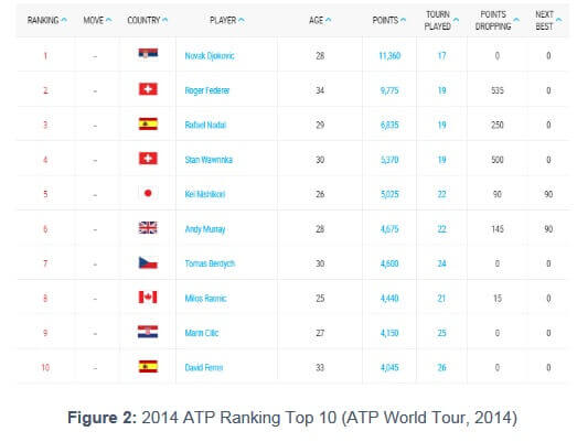
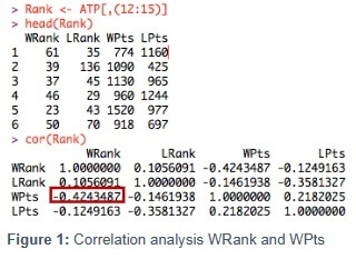This database contains information about the 2014 ATP season. Based on the factors listed previously, we only have information related to rankings. In this regards, we can state that there is a correlation between the ranking position (WRank) and the ranking points (WPts) in the sense that the highest rank player will have the highest points. However, there is no strong correlation between the ranking position (N°1, N°2 & N°3 for example) and the number of points (11,360 pts, 9,775 pts & 6,835 pts respectively, see figure 1 and 2 ).

2.2 Correlation between the different odds

In order to avoid making use of two highly correlated variables, we first do a correlation analysis between the odds. Here we define all correlations above 0.85 as a high correlation. For the next chapter we can therewith avoid to use two highly correlated variables together in one regression analysis. This reduces redundancy and avoids that the algorithm provides irrelevant results by analyzing minor differences between these highly correlated variables. The correlation analysis offers the results below :

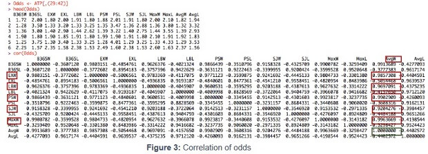
2 Figure 2 : 2014 ATP Ranking Top 10 (ATP World Tour, 2014) 2 .2 Correlation between the different odds In order to avoid making use of two highly correlated variables , we first do a correlation analysis between the odds. Here we define all correlations above 0.85 as a high correlation. For the next chapter we can therewith avoid to use two highly correlated variables together in one regression analysis. This reduces redundancy and avoids that the{" "} algorithm {" "} provides irrelevant results by analyzing minor differences between these highly correlated variables. The correlation analysis offe rs the results below : Figure 3 : Correlation of odds As in the following regressions the Average o dds of match winner (AvgW) will play an important role, the figure above shows all the variables that are highly correlated to it . Therewith, to give an example, we do not use Expekt odds of match winner ( EXW ) , Ladbrokes odds of match winner ( LBW ) , Pinnacles Sports odds of match winner ( PSW ) , Stan James odds of match winner ( SJW ) and M aximum odds of match winner ( MaxW ) as explanatory variables, when the average odds of match winner is the dependent variable. Due to the fact that they convey approximately the same information, it does not lead to meaningful results, if two of them g et used in the same regression.

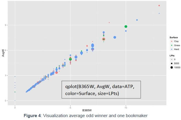
Figure 4 shows the relation of a bookmaker on the winner and the average odd winner. It appears as a linear function. Although some points might differ a bit, it is globally very similar, no matter the surface played or the ranking of the “Loser”.

3 Linear Multiple Regression

3.1 Entry Ranking of Winner as dependent variable

Prior to the regression analysis, we recoded several variables consisting of characters (Court, Surface, Round, Location and Tournament) in numerical variables. T o do so, we first had to transform them into factor variables and then into numerical variables (see annex 2 for codes).

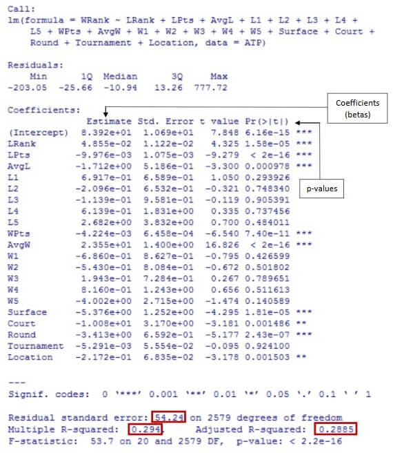
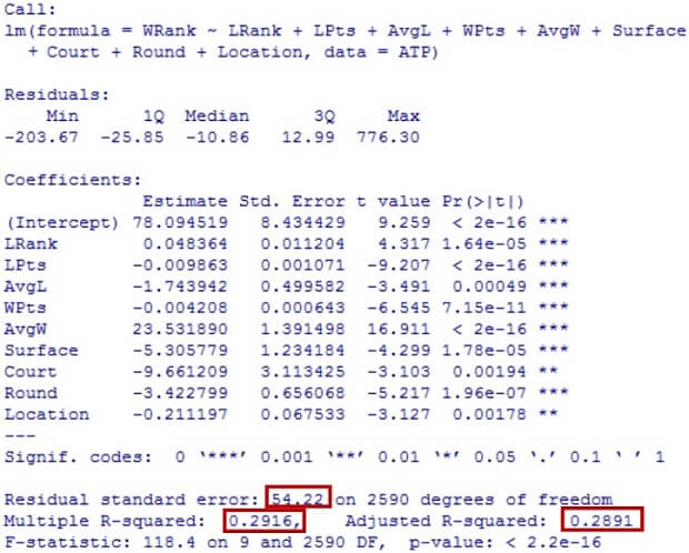
In order to see further relationships between variables, besides the correlations shown in the previous chapter, the following examination takes place in form of a linear multiple regressions . This analysis attempts to m odel the relationship between several explanatory variable s and a dependent variable. In the first trial we use the winner r ank before the match ( WRank ) as the dependent variable . As explanatory variables we chose to look at many different numerical variables (see annex 3 .1 ) and finally only kept the ones with a sufficiently small p - value. T he p - value stand s for probability value and is one of the outcomes of statistical tests when making a comparison. It evaluates if the estimate is significantly different from zero, thus if the variable is relevant in the model. The value is somew here between 0 and 1 and a p - value of e.g. “ 0 .015” indicates that the difference observed would only be seen about 1.5% of the time. Considered as statistically significant are p - values which are less than “0.05” (Sauro, 2015). Thus, only the estimates with p - values allowing a statistically significant result stayed in the regression and these are: LRank, LPts, AvgL, WPts, AvgW, Surface, Court, Round and Location (please see annex 1 for explanations regarding the abbreviations). This shows that there is a significant relation between the WRank and these explanatory variables. We explained in chapter 2.1 , that qplot(B365W, AvgW, data=ATP, color=Surface, size=LPts) 4 in practice there is a clear relation between WRank and WPts. Meaning as higher you are in the ranking (low numbers) as more poi nts you have (high numbers). The negative estimate WPts highlights this adverse relation. Figure 5 shows this relation and takes in consideration the Series and the Round. Low ranked player (>100) are playing first round of tournament while high ranked player (<50), starts l ater in the tournament. Furthermore, highest ranked player usually do not play small tournaments such as ATP250 Series. This is consistent with reality.

Another significant value is R², which is the percent of variance explained, meaning the fraction by which the variance of the errors is less than the variance of the dependent variable. Usually a valid R² should be somewhere greater than 50%. After the analysis we can see that we have a R² of 0.2917, which is rather low. The adjusted R² equals to 0.2891 and the standard error is 54.22 on 259 0 degrees on freedom. This standard error is quite high.

Generally speaking, it is recommend to look at the adjusted R² and at the standard error of the regression. These are unbiased estimators, which correct for numbers of coefficients estimated and for the sample size. The adjusted R² is most often a little bit smaller than the R ² ( Nau, 2015 ). The standard error indicates the average distance that the observed values fall from the regression line. It shows how wrong the regression model is on average using the units of the response variable. As smaller the values are as better, as then the observations are closer to the line (Frost, 2014). So this analysis shows, that even though we have significant estimates, the model is not completely trustworthy. The code and the detailed results are shown in annex 3.2.

3.2 Average betting odds as dependent variable

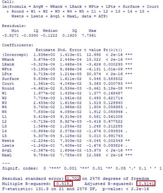
To provide a broad analysis of the relationship among dependent and explanatory variables we have conducted a second trial. This linear multiple regression will try to explain another qplot(WRank, WPts, data=ATP, color=Series, size=Round) 5 hypothesis and its variation with the inclusion of the Average odds of match w inner (AvgW) as our dependent variable and several explanatory variables that are presumed to influence our variable (see annex 4 ). In other words, we will try to prove if the Average betting odds are mainly related to the WRank and WPts ( p lease refer to annex 1 for abbreviations ) or on the opposite it depends of outsider variables such as the Location, Surface or Tournament (see anne x 4.1 for code).

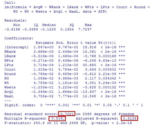
After the analysis we notice the strong influence of variables such as WRank, WPts, Wsets among other s that where considered due to their significant estimates and low p - values (see annex 4.2 ) As previously stated, a low p - value ( less than 0.05 ) indicates that we can reject the null hypothesis (Frost, 2014). Moreover, keeping the variables with low p - values are likely to be meaningful for our model variable because it means that changes in the dependent variable are related to changes in the response variable s. Essentially, the average betting odds evidence a significant relation among WRank, Location, Court and its other variables in reasonable proportions. Our regression has a percentage of variance or R² of 0. 516 which is an a dmissible value considering that R²{" "} represents how close is the data to the fitted linear regression (Frost, 2014). Even though, results over 50% are preferred in order to be an acceptable value it should be over 55% meaning that the higher the R², the better the model fits the data. With an adjusted R ² of 0.5139 and a residual standard error of 0.7021 with 2588 degrees of freedom which is reasonably small, indicating that this hypothesis over the variables related to the Average odds of match winner (AvgW) fairly fits the data. This analysis allows us to conduct further examinations, this time considering this variable as valuable for our hypothesis.

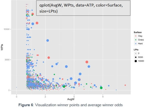
Figure 6 highlights the relationship between WRank (here symbolized by number of points) and the average betting odds: the highest the points, the smaller the rate.

3.3 Average betting odds divided by Winner Points as dependent variable

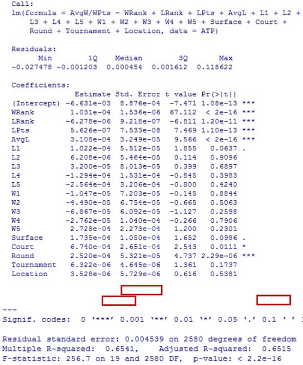
In order to find the hypothesis with the closest dependent and explanatory variable relation we have conducted a third trial. This linear multiple regression tries to test the division of the previously analyzed variable, Average odd of match winner (AvgW) with Winner Points (WPts) as a possibly related variable. We chose to divide AvgW by WPts, as it was one of the strongest estimates in the previous analysis. In this third regression, several explanatory variables were included to analyze its relation with the dependent variables ( see annex 5 .1 for variables and code).

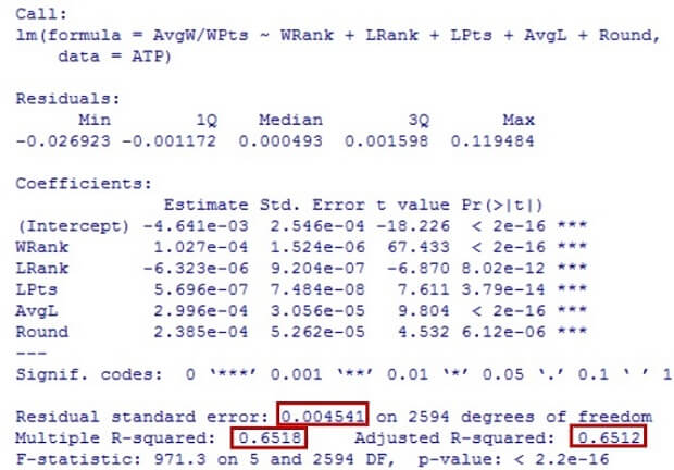
Once again, we have filtered the results only considering relevant coefficients and small p - values ( see annex 5.2 for results), we have kept the five explanatory variables with the lowest p - values for proving our hypothesis , which are : WRank, LRank, LPts, AvgL, Round. Our regression indicates a multiple R² of 0.6518 and an adjusted R² of 0.6512. The R² is thus 65.18%, which represent s 10.18% over the 55% average, which proves that w e have obtained satisfactory values that explains the fitting of the data even better than our two previous trials. T his means that there is a positive reaction with the measure of AvgW and WPts with other variables such as the WRank or LRank. Apparently, the Average odd winner (AvgW) is considering the player ’s W inner points (WPts) and is influenced by the points on the Ranks (WRank and LRank) and the amount of Rounds. This hypothesis can be proved to fit our model looking at the value of the residual standard error . With a result of 0.00 45 41 over 2594 degrees of freedom it is a significantly low value that proves our observations to be really close to the line.

Figure 7 illustrates the influence of WRank and LRank on the ratio AvgW/WPts: the lower the rank, the higher the ratio. Interestingly, the match played on Clay seems to have a higher ratio.

The next chapter will analyze different trees based on the database we have used which regroups several factors values that can help better understand the ATP tennis environment.

4 Decision Trees

4.1 Determining the game winner

This tree shows which player is the most likely to win a tennis game based on the following variable: the winner ranking, the surface, the court, the series and the round ( annex 6 shows the factor variables). Indeed, we will see later in the results that a player can be displayed several times, which can be explained by his numerous number a matches played throughout the year and the evolving variables.

Figure 8 provides an insight of the result it displays (the full tree and formula used are shown in annex 7.1 ).

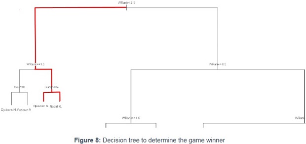
Focusing on the red path, going left (true side), only players ranked <2.5 (so either 1st or 2nd) at one point during the year 2014 will be match winners. Therefore, only three players have reached either 1st or 2nd (Federer, Djokovic and Nadal), but only one has been ranked >=1.5 (so 2nd): Federer, meaning that both Djokovic and Nadal have reached the N°1 spot during the year (right side of the path). To go beyond that, if we focus on the different surfaces (Clay, Grass and Hard), Djokovic is more likely to be the winner when the match will be played on Hard court (Djokovic led 15/8 on that surface at that point against Nadal and won all his 7 grand slams on hard court) as “Surface=c” indicates.

However when the match will be played either on Clay (his best surface: 9 French Open titles) or on Grass (Nadal won 2/3 matches on grass against Djokovic), Nadal will most likely end up as the winner.

4.2 Determining the winner ranking

On this tree, the focus is to find out the winner based on the average winning odd, the surface, the court, the series and the round. The red path will help us to better understand the logic of the ATP Ranking. Figure 9 provides an overview of the decision tree (the full tree and formula used are shown in annex 7.2).

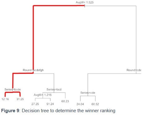
Focusing on the red path, going left (true side), only ranked players with an average winning odd <1.525 will appear in the results, in tennis language that would mean players ranked in the top 50 (players ranked above the 50th place will unlikely have an average winning odd <1.5, unless they play against a player ranked 300/400th in the world).

Then, the tree focuses on the round : again, going on the left side: here it would be for every round of a tournament except the 1st round (we assume that it is because sometimes players are exempt of 1st rounds due to their high ranking, which is called a “bye” in tennis ). After focusing on the rounds, the tree shows the ranking of the winner of the match based on the series, which are the different categories of tournament a player faces throughout the year (see f actor values for more details ). On the left side, series that include all tournaments except the ATP250 (the smaller tournaments in terms of fields, points, price money etc. ) that are shown on the right side.

If we take a look at the results, there is a logic behind each data: on the left side, the ranking of the winner is lower than on the left side, which means that the player who is more likely to win a match will held a quite high position in the ranking (12.16 in average). However, on the right side (which takes into consideration only ATP250), the ranking is higher (31.25) meaning that the winner of a match is not ranked as good, simply because the field of the tournament is weaker than in Masters 1000 or Grand Slam (more points, more price money) to name a few, where all top rank ed players will be in the draw.

4.3 Determining the average winner odd

In this tree, we will try to understand the aver age odd of an ATP match winner based on the winner points (in the ATP ranking), the loser points (in the ATP ranking), the surface, the court, the series and the round. Looking at figure 10 (the full tree and formula used are shown in annex 7.3 ), we see th at the first factor displayed is the loser points (<1354 pts). We will focus on the left side (true side) meaning focusing on match losers that have less than 1354 points in the ATP ranking, which are players ranked outside the top 30 in the ATP ranking.

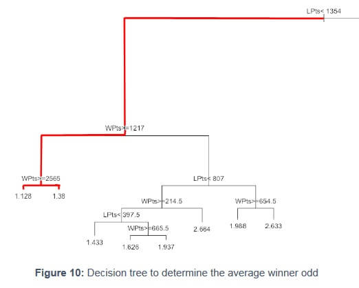
Then, if we keep following the red path, the tree identifies match winners that have at least 1217 points in the ATP ranking (left side), which are players inside the top 40. Last but not least, the red path identifies match winner that have at least 2565 points in the ATP ranking (left side), which are players inside the top 10. The winner average odd for a player ranked in the top 10 that plays against a player outside the top 30 (<1354 pts) is 1.128, which means that the top 10 player is the favorite of the match and that his chances to win are very high.

This can be explained by the huge gap existing not only in terms of ranking points but also in terms of level of tennis between the top 10 (and more precisely the top 4) and the players ranked outside the top 30. Indeed, between 2004 and 2014, all Grand Slam (40) have been won by players that were inside the top 10 (Federer, Nadal, Djokovic, Wawrinka, Murray and Del Potro).

5 Nearest Neighbor

Tennis often offers spectacular games, where players intensively dispute their chances. It sometimes leads to high score s in the last set in Grand Slams, except the USOpen where the final set is a tie break . The game between Wawrinka and Djokovic in Quarterfinals of the Australian Open is one of these games. At that time, Djokovic was ranked 2 nd and Wawrika 8 th.

As explained earlier, the betting odds depend on a certain number of variables. Considering especially the ranking of the two players and also the surface (Hard) of the game, the average odd for Wawrinka was 7.54. But as in every sport, everything can happen, and on that day, Wawrinka proved it by winning (2/6, 6/4, 6/2, 3/6, 9/7).

To us, it seems interesting to use the nearest neighbor approach to find similar games (9) and analyze the different variables. Although the approach aimed to consider the full database, considering “five sets” as variables to find similar match had a direct effect on the result. Indeed, we find only match from Grand Slam (best of five set s) tournaments. This is not surprising as the calculations are made with five sets and it explains why other disputed match from other tournaments (best of three sets) don’t appear in the top nearest neighbor.

Figure 12 provide s an overview of the indices, while annex 8 shows the detailed list and an nex 9 the script used.

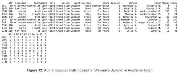
Looking closely to the rankings, we can see that it does not seem to affect the intensity of the contest. Although all Grand Slam are present in the list, there is only one Quarter finals. Especially the game between Murray and Kohlschreiber in Paris (12/10 in the last set) and the match between Kyrgios and Gasquet in London (10/ 8 in the last set ) look like very disputed.{" "}

Throughout this paper, the analysis of the dataset using correlations, regressions, decision trees and nearest neighbors, provided consistent results. Although some results seemed to be obvious and logical, we could verify the high correlations between the average odd and the bookmaker, the inversed correlation between the number of points and the ranking, and the relation between the ranking or points with the average odd.

Decisions trees enabled us to build on these findings to find out which player was the most likely to win in specific conditions, e.g., surface, ranking etc., what would be the ranking in specific conditions, e.g., odds, series, round etc., and what would be the odds depending on the players opposed and their respective points.

Finally, using the nearest neighbor approach provided us a list of nine similar games as the highly contested quarter finals of the Australian Open 2014 opposing Wawrinka and Djokovic.

7 Limitations

Along this project, we faced several limitations. First and foremost, the database possesses a lot of variables, but some of them could not be used for regressions due to the high correlations. Furthermore, it is about the ATP season and it provides information on the game, but do not look at the intrinsic qualities of each players. Having such variables a nd other external variables, e.g., weather, head to head and player’s trend could enable us to be more in the “predictive” analysis rather t han the “descriptive” analysis. Besides, we experienced also some limitations in terms of technic to improve the visualizations. For example, not considering some points, which are extremely high in Figure 7 , would have improve the scaling and therefore enhance the reader experience. In other plots also, and due to the database cleaning in excel, we would have like to remove all the “0” variables.

8 Conclusion

This database composed of 2600 instances and a total of 42 variables on the ATP season 2014 provided an excellent base for big data and analytics. Its specificities to report each game of the season with the respective betting odds, and updated ranking and points of each players, is precious to understand the impact of different variables, such as the ranking of each players, the series, the surface, the round, to determine the betting odds. Using different approaches is also an excellent way to have different insight about the ATP season.

Correlations and regressions are useful to understand how variables interact with each other while decisions trees are an excellent approach to determine a winner, a ranking or else, depending on these relations. Having a database on specific tennis skills could enable one to go further. Beyond, focusing on only one player along the season could also be interesting to see how variables evolve and if a specific opponent, regardless the ranking, is likely to influence the odds.

Bibliography

ATP World Tour (2014): ATP Rankings, available online: http://www.atpworldtour.com/en/rankings/singles?rankDate=2014-12-29, uploaded on 29.12.2014

BeatzeBook (2012): Cote Bookmaker,available online: http://www.beatzebook.com/cote-bookmaker.html, uploaded on 21.12.2012

Frost, Jim (2014): Regression Analysis: How to Interpret S, the Standard Error of the Regression, available online: http://blog.minitab.com/blog/adventures-in-statistics/regression-analysis-how-to-interpret-s-the-standard-error-of-the-regression, uploaded on 23.01.2014

Nau, Robert (2015): What’s a good value for R - squared? Available online: http://people.duke.edu/~rnau/rsquared.htm, last accessed on 13.01.2015

Pye, John (2014) : Australian Open: Novak Djokovic upset by Stan Wawrinka in quarter - finals , available online: http://www.thestar.com/sports/tennis/2014/01/21/australian_open_novak_djok ovic_upset_by_st an_wawrinka_in_quarterfinals.html , published 24.01.2014

Sauro, Jeff (2015): Customer Analytics for Dummies, John Wiley & Sons, Hoboken, New Jersey, February 2015, available online: http://www.dummies.com/how-to/content/statistical-significance-and-pvalues.html, last accessed on 13.01.2015

                    Sources of dataset: Tennis - data - http://www.tennis -
                    data.co.uk ATPtennis.com - http://www.atptennis.com/ ATP
                    Tour Rankings and Results Page -
                    http://www.stevegtennis.com/ Livescore -
                    http://www.livescore.net/ Oddsportal.com Xscores -
                    http://www.xscores.com/
                  

Annexes

Annex 1: Explanation of variables

Key to results data:

                    ATP = Tournament number (men) Location = Venue of tournament
                    Tournament = Name of tournament (including sponsor if
                    relevant) Data = Date of match Series = Name of ATP tennis
                    series (ATP250,ATP500,MastersCup,Masters 1000, Grand Slam)
                    Court = Type of court (outdoors or indoors) Surface = Type
                    of surface (clay, hard or grass) Round = Round of match Best
                    of = Maximum number of sets playable in match Winner = Match
                    winner Loser = Match loser WRank= ATP Entry ranking of the
                    match winner as of the start of the tournament LRank = ATP
                    Entry ranking of the match loser as of the start of the
                    tournament WPts = ATP Entry points of the match winner as of
                    the start of the tournament LPts = ATP Entry points of the
                    match loser as of the start of the tournament W1 = Number of
                    games won in 1st set by match winner L1 = Number of games
                    won in 1st set by match loser W2 = Number of games won in
                    2nd set by match winner L2 = Number of games won in 2nd set
                    by match loser W3 = Number of games won in 3rd set by match
                    winner L3 = Number of games won in 3rd set by match loser W4
                    = Number of games won in 4th set by match winner L4 = Number
                    of games won in 4th set by match loser W5 = Number of games
                    won in 5th set by match winner L5 = Number of games won in
                    5th set by match loser Wsets = Number of sets won by match
                    winner Lsets = Number of sets won by match loser Comment =
                    Comment on the match (Completed, won through retirement of
                    loser, or via Walkover)
                  

Key to match betting odds data:

                    B365W = Bet365 odds of match winner B365L = Bet365 odds of
                    match loser EXW = Expekt odds of match winner EXL = Expekt
                    odds of match loser LBW = Ladbrokes odds of match winner LBL
                    = Ladbrokes odds of match loser PSW = Pinnacles Sports odds
                    of match winner PSL = Pinnacles Sports odds of match loser
                    SJW = Stan James odds of match winner SJL = Stan James odds
                    of match loser MaxW= Maximum odds of match winner (as shown
                    by Oddsportal.com) MaxL= Maximum odds of match loser (as
                    shown by Oddsportal.com) AvgW= Average odds of match winner
                    (as shown by Oddsportal.com) AvgL= Average odds of match
                    loser (as shown by Oddsportal.com)
                  

Annex2: Recoding character variables in numerical variables

ATP$Court <-as.factor(ATP$Court)
ATP$Surface <-as.factor(ATP$Surface)
ATP$Round <-as.factor(ATP$Round)
ATP$Tournament <-as.factor(ATP$Tournament)
ATP$Location <-as.factor(ATP$Location)
i <-sapply(ATP,is.factor)
ATP[i] <-lapply(ATP[i],as.numeric)
summary (ATP[i])

Annex 3: Multiple Linear Regression with WRank

Annex 3.1: Code and results of regression with various variables Rank <-lm(WRank ~ LRank + LPts + AvgL + L1 + L2 + L3 + L4 + L5 + WPts + AvgW + W1 + W2 + W3 + W4 + W5 + Surface + Court + Round + Tournament + Location, data=ATP)
summary (Rank)

Annex 3.2: Code and results of regression with significant estimates

Rank <-lm(WRank ~ LRank + LPts + AvgL + WPts + AvgW + Surface + Court + Round + Location, data=ATP)
summary (Rank)

Annex 4: Multiple Linear Regression with AvgW

Annex 4.1: Code and results of regression with various variables

AvgWOdd <-lm(AvgW ~ WRank + LRank + WPts + LPts + Surface + Court + Round + W1 + W2 + W3 + W4 + W5 + L1+ L2 + L3 + L4 + L5 + Wsets + Lsets + AvgL + MaxL, data = ATP)
summary(AvgWOdd)

Annex 4.2: Code and results of regression with significant estimates

AvgWOdd <-lm(AvgW ~ WRank + LRank+ WPts + LPts + Court + Round + W3 + W5 + Wsets + AvgL + MaxL, data = ATP)
summary(AvgWOdd)

Annex 5: Multiple Linear Regression with AvgW/WPts

Annex 5.1: Code and results of regression with various variables

Rel <-lm(AvgW/WPts ~ WRank + LRank + LPts + AvgL + L1 + L2 + L3 + L4 + L5 + W1 + W2 + W3 + W4 + W5 + Surface + Court + Round + Tournament + Location, data=ATP)
summary (Rel)

Annex 5.2: Code and results of regression with significant estimates

Rel <-lm(AvgW/WPts ~ WRank + LRank + LPts + AvgL+ Round, data=ATP)
summary (Rel)

Annex 6: Factors values for decision trees

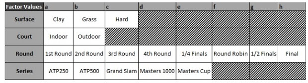
This table enables us to read the decision tree. For example, if one node is “Surface=c”, it means that “Hard” is true (left), and “Clay” and “Grass” are false (right).

The “character” variables were turned in numeric values using the formula “Database$Variable
<-as.factor(Database$Variable)” as follows:

• ATP$Round <-as.factor(ATP$Round)
• ATP$Surface <-as.factor(ATP$Surface)
• ATP$Court <-as.factor(ATP$Court)
• ATP$Series <-as.factor(ATP$Series)

Then, the order “a > b > c ...” can be obtained using summary(Database$Variable):

• summary(ATP$Round)
• summary(ATP$Surface)
• summary(ATP$Court)
• summary(ATP$Series)

Assignment Data Vizualization Fundamentals Tableau

IDEA Software Training Assignment

Accounts Receivable audit Assignment

ICT 300958 Social Web Analytics

Topics in database

• Authorization: SQL Recursion
• Big Data
• Database and data science techniques
• Database Languages Assignment Help{" "}
• Database Design Help
• Database System Architectures Design
• Entity Relationship Model Understanding
• Higher-Level Design: UML Diagram Help
• Implementation Of Atomicity And Durability{" "}
• Object-Based Databases Homework Help
• Oracle 10g/11g
• Parallel And Distributed Databases
• Query Optimization Technique{" "}
• {" "} Relational Databases Homework Help
• Serializability And Recoverability
• SQL Join
• SQL Queries And Updates
• XML And Relational Algebra Homework Help
• XML Queries And Transformations
• Data Mining
• Oracle Data warehouse
• Relational Model Online Help
• SQL And Advanced SQL Learning Help